Lua Scripting Example: Coil Gun
David Meeker
June 10, 2004
1. Introduction
This example considers the computation of the force on an iron ball at various positions relative to a wound, air-cored coil. The configuration is similar to some coil guns that are designed to shoot ball bearings. The specific configuration in pictured below in Figure 1.
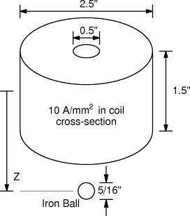
Figure 1: Wound coil acting on an iron ball.
In particular, this example is mean to demonstrate the following concepts in FEMM:
- Use of Lua scripting to accomplish a "batch" run;
- Use the Kelvin Transformation to accurately model an unbounded axisymmetric domain;
- Prescription of the current carried in a coil via the specification of current density;
- Use of the "Weighted Stress Tensor" integral to compute the magnetic force.
2. Problem Setup
In many instances, one would like to perform some sort of batch run in which perhaps one parameter in a problem is changed over the course of several program runs. When this is the case, it is typically advisable to draw the geometry from scratch inside a Lua script. It is typically easier to draw the geometry in the interactive FEMM preprocessor and change just the parameters of interest from run to run—this substantially simplifies the required Lua script.
An input geometry that describes the problem of interest is shown below in Figure 2. The iron ball is initially located 1.5" from the center of the coil.
Figure 2: Geometry in finite element
pre-processor.
2.1 Labeling of the Moving Parts
FEMM contains a notion of "group" membership. A group number is a label that can be applied to the various lines, arcs, and block labels in a geometry. The advantage of assigning entities to a group number is that then all of the members of the group can be selected with either a single click in the user interface or a single command in a Lua script. A second command can then be used to move all of the selected entites.l
To make it simpler to move the iron ball, all parts of the ball has been assigned to be members of group number 1. All other parts are members of group number 0, which is the default group number for entities that are not explicitly defined to be a member of a number group. It is relatively easy to assign a region to a given group. Put the preprocessor into group mode by pressing the "group" more button, as shown in Figure 3:

Figure 3: Group mode toolbar button depressed.
Then, group select all of the region of interest. Press the space bar button to "open" the group. A dialog will appear that will allow you to assign the group to which all selected entities are to be assigned.
2.2 "Open" Domain via the Kelvin Transformation
At first glance, it would appear to be impossible to represent an infinite exterior domain by finite elements. However, this not the case—in FEMM, it is simple to map an unbounded region onto a bounded one, such that the unbounded solution can be solved exactly without having to mesh a domain of infinite expanse. This mapping is known as the "Kelvin Transformation," and it is described in more detail in the references listed at the end of the paper.
For 2-D problems, setting up problems exploiting the Kelvin transformation is particularly easy. The "interior" region containing the items of interest and the air around them are placed inside one circle. A second circle is created and specified with air. However, the size and orientation of the second circle doesn't matter. This second circle represents the fields in the "exterior" region (i.e. the unbounded region filled with air). Periodic boundary conditions are then applied to the edges of the two circles such that the two circles are "linked" together at their edges. When the problem is solved, the correct solution is obtained (as if the interior region were actually located in an unbounded domain). If desired, fields throughout the exterior region could be inferred by applying a reverse mapping to the results, but the external field is typically not so much of direct interest.
For axisymmetric problems, things are a bit more complicated. Similar to the 2-D problems, the "interior" region is confined to the interior of a sphere. The "exterior" region is represented by a second coaxial sphere. Again, the edges of the interior and exterior regions are linked together using periodic boundary conditions. The difference is that in the axisymmetric case, the permeability of the exterior region must vary as a function of the distance from the center point of the exterior region (with permeability approaching infinity at the exact center of the mapped exterior region). FEMM takes care of varying the permeability in the axisymmetric exterior region in the appropriate way, but the program has to have a few extra pieces of information to do it. The Properties|Exterior Region selection from the FEMM main menu allows the user to enter the diameters of the interior and exterior region, as well as the position of the center of the exterior region along the z-axis, such that the program can compute the appropriate permeabilities to apply in the exterior region. Lastly, the block label(s) placed in the exterior region must be tagged as belonging to the exterior region. This is done via a check box in the block label properties dialog that pops up when a selected block label is opened.
The example at hand applies this axisymmetric Kelvin transformation approach to analyze the coil and iron ball as if they were placed in an unbounded domain. In this case, the small upper sphere represents the exterior region. Boundary conditions and Exterior Region properties have been properly defined in the example to yield an effectively unbounded domain solution.
2.3 Specification of Current in the Coil
Although FEMM contains the facilities to define the number of turns and the type of wire for a coil in a very detailed way, it is sometimes useful to define current-carrying regions in a simpler way, especially for magnetostatic problems at an early stage in the design process. An alternative way to specify currents is to specify the "source current density" for the material property that is assigned to the current-carrying region. The Amp*Turns is then the current density multiplied by the cross-section of the coil. This is the approach taken in the present example. A material called "Coil" has been defined with a source current density of 10 A/mm2. Multiplying by the cross-section of the coil would yield 9677.4 Amp*Turns.
3. Lua Script
In this case, it is desired to move the ball through a number of different position and report the result. In this case, the results will be reported to the Lua console screen, although it would also have been straightforward to write them to a temporary file. The complete Lua script is pictured in Listing 1:
mydir="./"
open(mydir .. "coilgun.fem")
mi_saveas(mydir .. "temp.fem")
mi_seteditmode("group")
for n=0,15 do
mi_analyze()
mi_loadsolution()
mo_groupselectblock(1)
fz=mo_blockintegral(19)
print((15-n)/10,fz)
if (n<15) then
mi_selectgroup(1)
mi_movetranslate(0,0.1)
end
end
mo_close()
mi_close()
Listing 1: Example Lua script.
First, the script shows the Lua console so that the results will be visible. The completed coil gun geometry is loaded into FEMM and then saved as a different, temporary, file name so that the original geometry is not subsequently over-written. The program then carries out a loop which performs the actual analysis and collects the results.
To evaluate the force, all elements associated with block labels in Group 1 (which we were using to represent parts of the moving ball) are selected using the mo_groupselectblock(1) command. Force is computed by invoking block integral 19, which returns the z-directed component of force from the "force via weighted stress tensor" computation. This integral is typically much more accurate either drawing a contour "by hand" and evaluating the magnetic shear along it, or by virtual work methods. The integral is essentially taking the average force due to many possible different stress tensor contours. In addition, these contours are automatically defined by the program and selected so as to be located in "well behaved" sections of the solution so that accuracy can be higher.
To run, select "Open Lua Script" from the File section of the FEMM main menu. Select the "coilgun.lua" script. The script will then evaluate the coilgun geometry at a number of different positions, displaying the force at each position to the Lua console. The series of 16 runs takes about 40 seconds total on a laptop running an AMD Athlon XP-M 2400.
4. Results
The plot of the calculated force on the ball versus position is pictured in Figure 4. The ball experiences the highest force just as it enters the coil.

Figure 4: Force on the iron ball versus position.
References
E. M. Freeman and D. A. Lowther, “A novel mapping technique for open boundary finite element solutions to Poissons equation,” IEEE Transactions on Magnetics, 24(6):2934-2936, November 1988.
D. A. Lowther, E. M. Freeman, and B. Forghani, “A sparse matrix open boundary method for finite element analysis,” IEEE Transactions on Magnetics, 25(4)2810-2812, July 1989.
E. M. Freeman and D. A. Lowther, “An open boundary technique for axisymmetric and three dimensional magnetic and electric field problems,” IEEE Transactions on Magnetics, 25(5):4135-4137, September 1989.
Companion Files:
https://www.femm.info/examples/coilgun/coilgun.lua
https://www.femm.info/examples/coilgun/coilgun.fem
Mathematica version of the Coilgun script. Includes comparison with an analytical solution.
PDF Printout of Mathematica Coilgun script.