Rotating Losses in a Outrunner Doubly Salient Permanent Magnet Generator
David Meeker
dmeeker@ieee.org
09Sept2009
Companion Files: getloss.zip
1 Introduction
This note will consider the analysis of an "outrunner" (rotor on the outside) single-phase doubly salient permanent magnet machine. This machine is interesting from the point of view of core loss computation because the rotor and stator iron are both laminated and see different dominant frequencies. This example will show how a series of FEMM solutions (e.g. a simulation at one degree steps around an entire rotation) can be used to compute core losses in this challenging structure. Matlab scripts will be used to control the series of batch FEMM runs. The scripts will also collect information that will allow a simple circuit representation of the machine to be developed. Mathematica versions of the scripts are also included in the getloss.zip distribution.
2 History of Single Phase Doubly Salient Machines
An interesting type of permanent magnet machine is the single-phase "doubly salient permanent magnet" machine. Perhaps the first version of this machine is a linear motor, usually known as the Sawyer Motor. Although the Sawyer motor is usually configured as a two-phase device, the motor, as originally envisioned in US Patent 3,457,482 (filed in 1967) has two essentially independent phases spatially positioned 900 out of phase. Each individual phase looks as shown in Figure 1.
Figure 1: One phase from the Sawyer motor pictured in US patent 3,457,482.
In the machine shown in Figure 1, a mover consisting of a magnet, two iron cores, and a single coil travels above a toothed iron track. Since same amount of iron pole area is covered regardless of the mover's position, cogging force is relatively small. As the mover travels over the track, the flux from the permanent magnets is shunted between the left and right sides of either pole, driving the flux linking the coil between positive and negative extremes as the mover travels over its track.
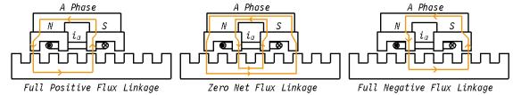
Figure 2: Sawyer motor flux versus position.
Since linear motors are essentially unrolled rotating motors, the Sawyer motor implies a related rotating machine. "Inrunner" (machines with the typical stator-on-the-outside/rotor-on-the-inside configuration) versions of the Sawyer motor has been patented as US patents 5,672,925 and 6,342,746.
3 "Outrunner" Machine
Although "inrunner" single-phase DSPM machines have previously been considered, it might also be useful to have an "outrunner" version, where the rotor is on the outside of the machine and the stator is on the inside. For example, some small gasoline-powered generator designs use an outrunner machine for the generator, letting the rotor also act as a flywheel. If an outrunner configuration is assumed it is straightforward to use the original Sawyer motor design in Figure 1, which features a simple configuration with just one coil and one magnet, whereas inrunner machines typically employ multiple magnets and coils. An example of this outrunner layout is shown in Figure 3. This outrunner DSPM will be considered for the purposes of the present example.
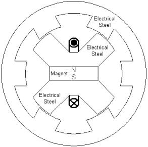
Figure 3: "Outrunner" single-phase DSPM machine layout.
3.1 Machine Performance Specifications
For the purpose of posing a specific example problem, it is assumed that the objective is to construct a generator to be attached to a small portable gasoline engine. The desired performance is summarized in Table 1.
| Parameter | Value |
| Generator Speed | 5000 RPM |
| Design Power Output | 500W |
| Nominal Output Voltage | 48Vpk |
Table 1: Generator performance specifications.
3.2 Example Machine Geometry
The dimensions of a particular example machine are pictured below in Figure 4. All dimensions shown are in units of millimeters. Additional attributes not pictured on Figure 4 are listed in Table 2.
| Parameter | Value |
| Axial length of rotor | 60 mm |
| Lamination material | DI-MAX M-19 Silicon Steel |
| Lamination thickness | 0.18 mm (7 mils) |
| Lamination stacking factor | 92% |
| Magnet material | N35SH |
| Number of turns | 40 |
| Wire | 8 strands of 24 AWG copper wire |
Table 2: Additional Machine Parameters.
Typically, one would solve a thermal problem in conjunction with a magnetic problem to find the temperature distribution corresponding to the nominal operating point. For simplicity, however, it will be assumed for this example that the average temperature of the windings at the desired 500W/5000RPM operating point is 700C and the average temperature of the magnet is 600C. The elevated temperature increases the resistivity of the winding, leading to additional loss. The increase in temperature also affects the magnets, lowering the energy product versus their rated energy product at room temperature.
Figure 4: Example machine dimensions in mm.
4 Electric Circuit Model
The objective is to calculate the core loss of the machine under load. However, the exact operating conditions under load are not clear a priori. The load that the generator drives, in combination with the generator's electrical characteristics, determines the operating condition. By making a circuit model of the machine under load, the operating point at which to analyze losses can be determined.
As an initial model, (that, for the moment, neglects core losses), the circuit model pictured in Figure 5 will be assumed. This model consists of a voltage source that is proportional to the rotor's speed (flux linkage, &lambda multiplied by the number of poles on the rotor, n, times the rotational speed &omega in units of radians/second); an internal inductance, L, and an internal winding resistance, Rs. To back out the operating condition for the determination of losses, a series of finite element runs can be performed, and best-fit parameters can be regressed.
Figure 5: Simple generator circuit model.
One complicating factor in determining the inductance is the presence of the permanent magnet. Typically, one can find inductance of a coil by doing a simulation with current in the coil, applied via a "circuit property." The "flux/current" obtained by viewing the circuit's properties in the postprocessor can then be taken as inductance. However, if there is a permanent magnet, some of the linked flux is due to the permanent magnet, so assuming that "flux/current" is the same as inductance would lead to large errors in the estimation of inductance. To get the incremental inductance about an operating point established by the permanent magnet, the best way is to compute the flux linkage for a small positive-valued current and a small negative-valued current. The inductance can then be taken as the change in flux linkage divided by the difference of the two test currents.
So as not to have to perform a third calculation for flux linkage just due to the magnet, it is reasonable merely to take the average flux linkage of the two calculations with perturbation currents.
The results for incremental inductance versus position are shown in Figure 6. The results for PM flux linkage versus position are shown in Figure 7. A Matlab script that evaluates the inductance and flux linkage is included as rolled_inductance.m.
Figure 6: Inductance versus angular position
Figure 7: Flux linkage versus angular position
The best-fit values for inductance and flux linkage amplitude are:
L = 0.001770 H
λ = 0.01619 Wb
To obtain a reasonable value of coil resistance, end-turn resistance must also be taken into account, and the increase in resistance due to temperature rise of the winding must be considered. FEMM reports the resistance (in "Circuit Properties") to be 0.0601774Ω, a result that does not account for end turns, but which does account for a 500C temperature rise in the winding. (Determining the temperature rise in the winding is usually its own elaborate calculation. For the purposes of this analysis, however, a particular temperature rise is simply assumed as a placeholder). For the purposes of estimating a value of end turn resistance, we could assume that the center of the winding is at a height of approximately 14 mm. If it is assumed that the end-turns have a roughly half-circle shape on each side, the mean end-turn would have a length of π * 14 mm = 44 mm. The depth specified for the problem in the into-the-page direction is 60 mm, so a reasonable estimate of the resistance would be to multiply the nominal resistance by (60mm + 44 mm)/(60 mm) = 1.73, which yields an estimated resistance of:
Rs = 0.104307Ω
It is interesting to note that the inductance is relatively huge in this machine. A large inductance appears to be a general attribute of this class (i.e. "flux switch", "flux reversal", "doubly salient permanent magnet", etc.) of machine. At 500Hz (the electrical frequency corresponding to a mechanical speed of 5000 RPM for this six-legged rotor machine, i.e. ω = n ωr), the reactive impedance is:
Zreact = ω L = (3142 rad/s)*(0.00177H) = 5.566Ω
The no-load voltage amplitude generated by the machine is:
V = ω λ = 50.86 V
The desired output is 500W, which implies that a current amplitude of about 20A would be required to obtain a 500W output. However, the voltage drop over just the internal reactance for a 20A current is about 111V--much larger than the ~51V available from the generator.
The circuit model implies that reactive power compensation is necessary to realize the desired output. At 500 Hz, the capacitor that balances out the machine's inductance is:
C = 1/(ω2 L) = 57.2 μF
A motor run capacitor could be used to nearly cancel out the reactive impedance of the machine at the running speed. It should be noted, however, that the capacitor will only provide good reactive power compensation at one running speed, not across a variable speed operating range.
5 Core Loss Model
There are a number of methods for estimating the core losses of an electric machines. As explained in [1] and [2], a consistent way is to incorporate a model of the core loss mechanisms (eddy currents, hysteresis, and excess loss) into the B-H relationship used in a time-transient model, such the effects of the core losses are directly visible as perturbations to voltage and current at the terminals of the machine. Unfortunately, it can be very difficult to create and time-consuming to run such a model. A commonly used alternative approach (referred to as the "Traditional Technique" in [1]) is to infer an estimate of core losses from the post-processing of a series of essentially magnetostatic runs that ignore the loss mechanisms in the computation of the magnetic field. This approach assumes that because the core is laminated, the core losses will have only a small effect on the field distribution so that reasonably accurate estimates of the field distribution can be obtained by neglecting losses.
In the "Traditional Technique," losses are then inferred from the computed magnetostatic field distribution using experimentally obtained loss data. To aid in the application of this experimental data, it is useful to fit the experimental loss data to a simple, empirical, functional form so that the losses can be quickly evaluated given a particular flux magnitude and frequency. This section will take core loss data from manufacturer's data sheets and converts it into an empirical form that can be directly applied to core loss calculations.
5.1 Core Loss Data
Material property data is required as a basis for core loss calculations. A grade of silicon core iron that is both high quality and commonly available is M-19. Loss data for M-19 is shown below in Figure 8 for a 29-gauge sheet (0.014" thick).
Figure 8: Core loss curves of 29-gauge sheet.
For the purposes of loss computation, it is useful to have a simple form that approximately captures the entire range of curves. A "traditional" way to do this is to assume that the loss can be broken into a part due to hysteresis, which varies linearly with frequency, and a part due to eddy currents, which varies with the square of frequency:
| P = Ph + Pe = Chω B2 + Ceω2 B2 | (1) |
where Ph and Pe are hysteresis loss and eddy current loss, respectively. Parameters Ch and Ce are hysteresis and eddy current loss coefficients that are regressed from the core loss data. The B in the formula is the amplitude of the flux density (i.e. the peak value).
A reference for the "classical" derivation of core loss separation is [3]. A more modern discussion is contained in [4]. The simple form of (1) is employed here because a curve fit to this form yields reasonable accuracy over the range of application in the problem under consideration.
A reasonable fit to the data for 29-gage M-19 from 50Hz to 600 Hz is:
| Ch = 0.00844 Watt/(lb*Tesla2*Hz) |
| Ce = 31.2*10-6 Watt/(lb*Tesla2*Hz2) |
For the purposes of finite element calculations, however, we are interested in loss per unit volume, not loss per unit weight. The density of M-19 is:
ρ = 7.70 gm/cm3
If the density is used to convert between loss per unit weight and loss per unit volume, the loss is:
| Ch = 143 Watt/(m3*Tesla2*Hz) |
| Ce = 0.530 Watt/(m3*Tesla2*Hz2) |
5.2 Extrapolation of Core Loss to 7 mil Lams
The machine under consideration employs 7 mil (0.18 mm) thick laminations. These relatively thin laminations are required because the machine runs at a relatively high electrical frequency (500 Hz vs. 50 or 60 Hz for most electric machines). Unfortunately, the core loss data in hand does not consider 7 mil laminations. However, the performance of a 7 mil lamination can be estimated from the loss separation empirically identified for the 29 gauge (14 mil) lamination. As the lamination thickness changes, the hysteresis loss is expected to remain more or less constant. However, the eddy current loss is theoretically expected to vary with the square of lamination thickness. Since, going from 14 to 7 mils, the lamination thickness is cut in half, the eddy current coefficient should drop by a factor of 4, whereas the hysteresis coefficient should remain constant. The extrapolated loss characteristics of 7 mil M-19 are:
| P = (143 ω B2 + 0.132 ω2 B2 ) W/m3 | (4) |
where, for the purposes of the formula, is in Hz and B is the peak flux density in Tesla.
To account for the stacking factor, it can be noted that the entire loss (in this estimate) scales by B2. We'd expect that the concentration of flux would increase the loss inside the lamination by (1/StackingFactor)2. However, the iron per unit volume also goes down—there's less iron per unit volume to generate losses, which gives back a factor of StackingFactor. Overall, the stacking factor can be incorporated in the loss by simply dividing the loss formula by the stacking factor of 0.92:
| Pstack = (155 ω Bm2 + 0.143 ω2 Bm2 ) W/m3 | (5) |
Eq. (5) is the equation to use for loss per volume in the machine under consideration.
5.3 Multiple Harmonics
The flux versus time predicted by the finite element model will not be sinusoidal, because it will be including all effects of the motor's geometry as the rotor moves past the stator. If the stator steel were described by linear material properties, the losses could be rigorously decomposed into elements occurring at different frequencies which are summed to obtain the total loss. Even though the material properties are not linear, a widely used an approximate method of estimating core losses is to assume that the losses can still be decomposed into multiple components occurring at multiple time harmonics. The core loss expression can then be applied to the each harmonic and the results summed to obtain an approximation of the total core loss. Mathematically, this approach can be represented as:
| (6) |
where Bm is the amplitude of the mth time harmonic of the base frequency, ω. It is (6) which will be directly applied, in the next section, to calculate core losses.
6 Loss Calculation
Equation (6) is the basis for computing loss in the machine's laminations. However, many finite element runs must be performed to collect the information necessary to apply (6) throughout the machine so that the total losses can be computed. The mo_numnodes, mo_numelements, mo_getnode, and mo_getelement commands that were added in the 15Jul2009 release of FEMM provide the element-level access to the mesh that is necessary to keep track of the flux density vs. rotor angle in each element of the laminated iron.
To collect and analyze the requisite flux density vs. time information, a (heavily commented) Matlab script was created (rolled_getloss.m). The script performs a series of finite element runs, incrementing the rotor position and stator currents with each successive run.
During the first run of the series, the script performs some additional bookkeeping that is needed to locate the points at which the magnetic field is to be evaluated during subsequent iterations of the script. The location of the centroid and the size of each element contained in a laminated region is recorded for later use. As the rotor's position is changed, the finite element mesh changes. The element centroids from the initial finite element mesh are fixed points in the lamination geometry at which the field is evaluated in each incremental analysis, regardless of remeshing.
The flux density is then evaluated at every stored element centroid for every rotor position, essentially building up a history of flux density versus time for each element in the laminated regions. Some extra care is required for points located in the rotor. The initial centroid locations need to be rotated through the same angle as the rotor so that the rotor field is always evaluated at the same points on the rotor from run to run. The resulting field evaluations also need to be rotated so that the field is for points on the rotor is always represented in the same rotor-fixed reference frame.
Once finite element runs have been performed over an entire rotation, Matlab's built-in Fast Fourier Transform (fft) function is used to turn what is essentially a time series of flux densities at each element centroid into amplitudes of various harmonics of flux density, as required by (6) for the evaluation of losses. The contributions from all harmonics for all elements are then added up to get the total core loss.
Running the core loss script with a coil current amplitude of 20A positioned in-phase with the no-load voltage (i.e. more or less the rated current, assuming that there is a capacitor that balances all of the reactive power of the generator), the script produces the following results:
Core loss: 20.9223 W
Core loss density: 7.8972 W/lb
Average torque: -0.9649 N*m
Rotor speed: 5000 RPM (523.6 rad/s)
Mechanical power: -505.2136 W
The script can be run at various currents to map out the behavior of core loss versus load current. The resulting curve of core loss versus load current, assuming that the load current is in phase with the no-load voltage, is shown in Figure 9.
Figure 9: Core loss for various load currents.
7 Circuit Model Including Losses
To explore the operation of the generator under different loads, it is useful to have a version of the simple circuit model that incorporates extra impedances to model the losses. In this way, the effects of the losses at the terminals of the machine can also be modeled in a consistent way (at least, in the context of the simple circuit model). A candidate circuit that models core losses is shown in Figure 10. An extra resistor, Rc, shunts off some current from the load, producing losses. It can be noted that since this this resistor is in parallel with the load, it can produce losses in the machine even when the machine is unloaded. The use of an extra parallel resistance to represent core loss is fairly commonplace, especially in the context of transformers.
To fit the losses produced by the circuit model to the losses computed from the finite element runs, it is assumed that the loss resistor splits the machine's inductance into two parts, L1 and L2. The split of the inductance between L1 and L2 and the value of Rc are then determined on the basis of a least-squares fit between losses predicted by the circuit model and losses predicted by the finite element model for the same load current. The best-fit parameters are presented below in Table 3. Such a circuit could then be used, for example, in a Spice simulation of the generator driving a reactive power compensation capacitor in series with a battery charger.
Figure 10: Equivalent circuit with core loss model.
| Parameter | Value |
| L1 | 0.632 mH |
| L2 | 1.138 mH |
| Rc | 97.70 Ω |
| λ | 0.01619 Wb |
| Rs | 0.104307 Ω |
| n | 6 |
| ωr | 523.6 rad/s |
Table 3: Circuit parameters for equivalent circuit including core losses.
8 Conclusions
An example has been presented in which FEMM is used compute the core losses of an electric machine under load. In the machine considered in this example, only coil resistive losses and core losses in the machine's laminate iron were considered. A more complete analysis also would have considered the generation of eddy currents in the permanent magnets (which could be added to the loss calculation script in a straightforward way) and windage/bearing losses. A more complete thermal analysis of the motor would also help to determine the actual operating temperature of the machine, which influences the resistance of the windings and the flux sourced by the permanent magnets.
The use of FEMM to identify parameters in simple circuit representations of electric machines has also been considered. The use of circuit representations can help to identify the operating conditions for which the finite element analyses are to performed, and circuit representations can lend intuitive insight into the design and operational attributes of the machine under analysis.
Although the specific machine considered in this example is of an unusual (and, perhaps, impractical) design, the scripts used to compute the core losses for this machine should be readily adaptable for use in other machine geometries.
References
[1] E. Dlala, "Comparison of models for estimating magnetic core losses in electrical machines using the finite-element method," IEEE Transactions on Magnetics, 45(2):716-725, Feb. 2009.
[2] H. Trabelsi, A. Mansouri, and M. Gmiden, "On the no-load iron losses calculations of a SMPM using VPM and transient finite element analysis," International Journal of Sciences and Techniques of Automatic Control & Computer Engineering, 2(1):470-483, July 2008.
[3] R. L. Stoll, "The analysis of eddy currents," Oxford University Press, 1974.
[4] D. M. Ionel et al. "On the variation with flux and frequency of the core loss coefficients in electrical machines," IEEE Transactions on Industry Applications, 42(3):658-667 May/June 2006. (http://eprints.gla.ac.uk/3438/)