FEMM 4.2 Electrostatics Tutorial
David Meeker
dmeeker@ieee.org
revised December 31, 2014
1 Introduction
Finite Element Method Magnetics (FEMM) is a finite element package for solving 2D planar and axisymmetric problems in electrostatics and in low frequency magnetics. The program runs under runs under Windows 2000, XP, 7, and 8, as well as on Linux machines via WINE. The program can be obtained via the FEMM home page at http://www.femm.info.
The package is composed of an interactive shell encompassing graphical pre- and postprocessing; a mesh generator; and various solvers. A powerful scripting language, Lua 4.0, is integrated with the program. Lua allows users to create batch runs, describe geometries parametrically, perform optimizations, etc. Lua is also integrated into every edit box in the program so that formulas can be entered in lieu of numerical values, if desired. (Detailed information on Lua is available from http://www.lua.org/manual/4.0/). There is no hard limit on problem size—maximum problem size is limited by the amount of available memory. Users commonly perform simulations with as many as a million elements.
The objective of this document is to get new users “up and running” with the program via a set of step-by-step example electrostatics problems.
2 Basic Introduction: Capacitor with a Square Cross-Section
This will take you through a step by step process of analyzing a capacitor with a square cross-section. Users should first refer to the FEMM user’s manual regarding the general interface(i.e. keyboard and mouse controls).
This example, as shown below in Figure 1, the outer square has a 4 cm size and the inner square has a 2 cm size. The geometry extends for 100 cm in the “into-the-page” direction. The dielectric between the plates is air. We seek to build the problem, analyze it, and determine the capacitance.
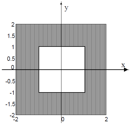
Figure 1: Square Cross-Section Capacitor
Because of the symmetry, only one quarter of the device need be modeled. The finished model will look as pictured below in Figure 2 when ready for analysis.
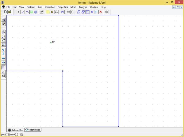
Figure 2: Completed example in the electrostatics preprocessor.
The steps required to create this model are as follows:
2.1 Create model
Start FEMM by select the "femm 4.2" entry placed in the "femm 4.2" section of your start menu.
After the program starts, "File | New" from the main menu. Select "Electrostatics Problem" in the "Create a new problem" dialog that appears. After you hit "OK", a blank electrostatics problem will appear.
Select “nodes” from the tool bar (this is the farthest button on the left with a small black box:
 ) and place 6 nodes for the corner of a box (at, for example, (0,1), (1,1), (1,0) ,(2,0),(2,2) and (0,2)). One can place nodes either by moving the mouse pointer to the desired location and pressing the left mouse button, or by pressing the <TAB> key and manually entering the point coordinates via a popup dialog.
 Select “lines” from the tool bar (second button from the left with a blue line:
 ). To select a node to be the endpoint of a line, click near each desired endpoint with the left mouse button. Select connect the points as pictured in Figure 2 using this mouse endpoint selection approach.
 2.2 Add materials to the model
Select “Properties | Materials” off of the main menu. In the dialog that appears, click the “Add Material” button. A dialog will pop up with edit boxes for the various material properties. Change the name of the property from “New Material” to “air.” By default the permittivity of a new material is 1, which is what we require for air. Press the “OK” button to complete the creation of the material.
2.3 Define materials for each region
Now click on “Block Labels” (the tool bar button with green circles
 ), and place a block label in the middle of the solution domain, between the inner and outer squares. Like node points, block labels can be placed either by a click on the left mouse button, or via the <TAB> dialog.
 Right click on the block label node for the outer box so that the node turns red, denoting that it is selected. Press space to “open” the selected block label. A dialog will pop up containing the properties assigned to the selected label. Set the “Block type” to “Air”. When the “Let Triangle choose Mesh Size” box is checked, the mesh generator is free to pick its own element size. The default mesh size is sufficient for many problems. However, if you desire a finer mesh, you can uncheck the “Let Triangle choose Mesh Size” checkbox and manually enter a value for “Mesh size”. The mesh size parameter defines a constraint on the largest possible elements size allowed in the associated section. The mesh generator attempts to fill the region with nearly equilateral triangles in which the sides are approximately the same length as the specified “Mesh size” parameter.
Define Conductor voltages
Select “Properties | Conductors” from the menu bar, then click on the “Add Property” button.
Replace the name “New Conductor” with “zero”. Select the “Prescribed Voltage” radio button. Enter a 0 as the value in the associated edit box and Hit “OK”. You have just defined a conductor that is fixed a voltage of 0V, but you have yet to assign this condition to a particular part of the model.
Repeat the above process but instead name the new boundary condition “one” and apply enter a prescribed voltage value of 1.
Select “lines” from the toolbar then right click on the each of the two segments belonging to the inner conductor. When a segment turns red, you have selected it. Now press space bar and the “Segment Properties” window will appear. From the “In Conductor” drop box change the selection from “<None>” to “one”. Repeat this process for the outer conductor, but set the conductor type to “zero”.
(N.B. for arcs or segments with a prescribed voltage, it is permissible to define a “Fixed Voltage” boundary condition in lieu of defining a fixed-voltage conductor property. The advantage of defining the boundaries as conductors, rather than simple boundary conditions, is that charge on the conductor is calculated automatically in the solver.)
2.5 Set Problem Characteristics
Select “Problem” from the menu bar. In the dialog that appears, make sure the problem type is “planar”. Set the length units to “Centimeters” and set the “depth” parameter to 100. The default solver precision of 10-8 (i.e. solution determined to single precision accuracy) generally need not be modified. If desired, a descriptive commend can be added in the “Comment” edit box.
2.6 Generate Mesh and Run FEA
Now save the file and click on the toolbar button with yellow mesh:
 . This action generates a triangular mesh for your problem. If the mesh spacing seems to fine or too coarse you can select block labels or line segments and adjust the mesh size defined in the properties of each object. When you are satisfied with the mesh, click on the “turn the crank” button
  to run the FEA algorithm over your model.
 Processing status information will be displayed in a dialog box while the solver runs. If the progress bars do not seem to be moving then you should probably cancel the calculation. This can occur if insufficient boundary conditions have been specified. For this particular problem, the calculations should be completed in less than a second (although the solution time is highly dependent on the speed of the machine running the analysis). There is no confirmation for when the calculations are completed, the status window just disappears when the processing is finished.
2.7 Display Results
Click on the glasses icon
 to open the solution in a postprocessor window. The solution will then be displayed, as pictured in Figure 3. By default, a color density plot of voltage is displayed when the postprocessor starts. If desired, the default behaviors can be changed via the Edit | Preferences selection on the main menu of both the preprocessor and postprocessor. The charge on each conductor can then be determined by selecting View | Conductor Props off of the postprocessor main menu. A dialog will then appear that displays the voltage and total charge for each defined conductor. For the “one” conductor and with the default mesh size, the reported charge is 2.26651e-011 Coulombs. One can use the fact that charge is equal to the product of capacitance and voltage difference to determine the capacitance of the system. Since only ¼ of the total geometry is modeled, the total charge is 9.06604-011 Coulombs. In this case the voltage drop is 1 V, implying that the total capacitance is 90.66pF.
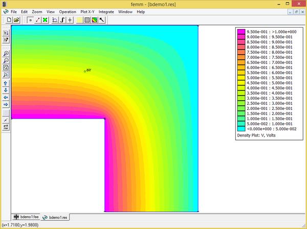
Figure 3: Solution to the example rendered in the electrostatics postprocessor.
From this basic introduction you should have gained the following principles:
- How to create your model space using nodes and lines.
- How to add material types to your model and how to assign them to regions.
- How to specify the finite element mesh size.
- How to define conductor properties for your model.
- How to apply conductor properties to line segments in the model.
- How to run the mesh generator and solver.
- How to run the postprocessor and display the resulting charge and voltage on each conductor.
A completed version of this example problem is available as bdemo1.fee
3 Additional Concepts: Capacitance between Two Spheres
You will now create a model of a capacitor consisting of two conducting spheres at equal and opposite voltages sitting in an unbounded region. This is an example of an axisymmetric system, and a special “open” boundary condition will be used to mimic the behavior of an unbounded domain.
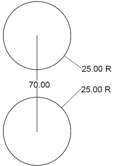
Figure 4: Two conducting spheres.
The arrangement of spheres is pictured in Figure 4. Two spheres, each 25 meters in diameter, are separated by a center-to-center distance of 70 meters. The top sphere is at a potential of 100 Volts, and the bottom sphere is at a potential of -100 Volts.
Due to symmetry considerations, only one sphere need be model. The line of symmetry between the two spheres is then fixed at 0 Volts to account for the effects of the second sphere.
We will use the “Asymptotic Boundary Condition” method (as described in the Appendix to the FEMM manual) to mimic an unbounded geometry. To apply this boundary condition, the finite element problem domain must be spherical (or circular for a 2D planar problem). When finished the modeled domain will look as pictured in Figure 5.
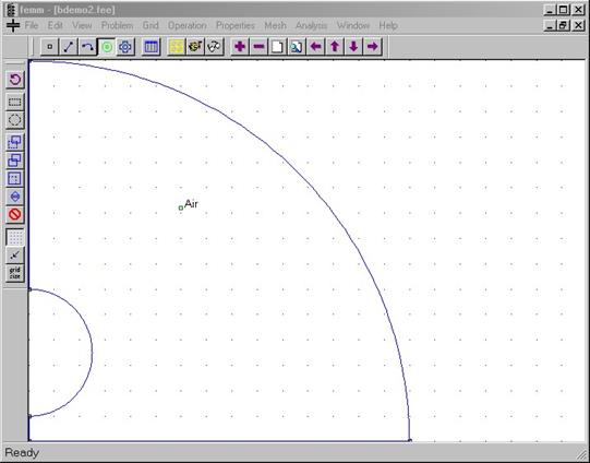
Figure 5: Example geometry shown in the electrostatics preprocessor.
First set the “Problem” properties to axisymmetric, and units of meters. Since the problem is axisymmetric, no Depth entry is required, and that edit box is grayed-out. In this case, the vertical axis is the axis of rotation for the problem. The r axis runs horizontally, and the z axis runs vertically.
Change the “Grid Size”
 to 10, meaning each dot
represents a 10 meter increment, and select snap-to-grid by pushing in the
 toolbar icon. Snap-to-grid allows points and block labels to be placed exactly on grid points using clicks of the left mouse button.
 Select View | Keyboard. This selection pops up a dialog allowing you to enter the size of the view via the keyboard. In this dialog, specify the lower-left corner of the screen to be at 0,0 and the upper right corner to be at (150,150). A view is then picked that contains the prescribed area as is best possible.
Place a nodes at (r,z) = (0,0), (0,10), and (0,60), (0,150) and (150,0) (refer to the left side of the status bar at the bottom of the screen for a read-out of the current mouse pointer position).
Connect lines from (0,0) to (0,10)and from (0,60) to (0,150). These lines are located along the axis of rotation for this axisymmetric problem. Also draw a line from (0,0) to (150,0), along the axis of symmetry between the two spheres.
Select the arc toolbar button
 . Select the (0,10) point (bottom point), then select the (0,60) point (top point). When the dialog box comes up, enter “180” for “Arc Angle” and “1” for “Max. Segment, Degrees”. The circles are ultimately represented as many-sided polygons, and the “Max. Segment” parameter prescribes the biggest arc that is allowed to be spanned by any one side of the polygon. A 1 degree constraint represents a fairly fine discretization—the default is 10 degrees. In the postprocessor, all arcs are drawn counter clockwise, so this will draw the halfcircle defining the outside of one of the conducting spheres.
 Now select the (150,0) point followed by the (0,150) point, and enter “90” for “Arc Angle” and “1” for “Max. Segment”. This arc will be the exterior boundary of the finite element solution domain.
Deselect “snap-to-grid,” switch to “block label” mode (by pressing
), and place a block label (green node) inside the closed region between the outer surface of the conducting sphere and the arc representing the exterior boundary Add “Air” to the model’s materials using the “Properties | Materials” main menu selection, as described in Example 1.
Select “Properties | Conductors” from the menu and create a conductor named “+100V” with a prescribed voltage of 100 Volts (procedure as described above in Example 1).
Create a fixed voltage boundary for the line of symmetry. Do this by selecting “Properties | Boundary” off of the main menu. Click the “Add Property” button and make a property named “zero” that has a prescribed voltage of 0.
Add a second block label that will be used as the condition on the exterior boundary. Rename your new boundary “open_bc” and change the “BC Type” to “Mixed”. Given that the system under analysis is close to the center of an arc (usually either a full or half circle), “c0 coefficient” can be set to (2εo /r ) where r is the radius of the arc in meters. In this case, you can let the program do the most of the appropriate calculations by entering the string:
2*eo/150
into the edit box for the c0 coefficient (the c1 coefficient should be zero). The quantity eo has been predefined to contain the permeability of free space in SI units, and we are exploiting the fact that the contents of every edit in FEMM box gets parsed by the Lua scripting language, enabling formulas to be entered in any edit box in which a numerical value is required.
Select the quarter-circle arc representing the exterior boundary by right clicking on or near it (the “Arc” toolbar button must also be depressed). Press space and assign the boundary condition to be “open_bc”.
Select the half-circle representing the surface of one of the conducting spheres. Press space and assign “+100V” as the conductor for property for this surface.
Switching to Segment mode, assign the “zero” boundary condition to the line of symmetry at z=0. In Block Mode, select the block label inside the domain by right clicking with the mouse near the green node. Change the “Block type” to Air and the “Mesh size” to 1.
Now generate the mesh, perform the calculation, and open the solution in a postprocessor window to display the resulting voltages, all in the same way as described in Example 1. The resulting solution should look as pictured in Figure 6.
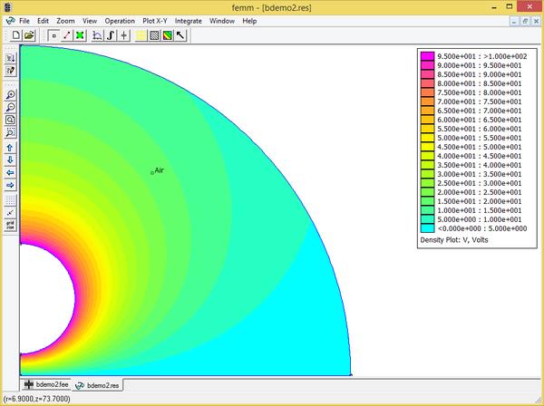
Figure 6: Solution to the example as rendered in the electrostatics postprocessor
Note that the vertical side of the semi-circle boundary (along the radial axis) does not have any boundary condition assigned—an “insulated” boundary condition is defined to the axis of rotation in axisymmetric problems by default. Also note how the equipotential lines radiate through the outer arc boundary as if heading to infinity. This is due to the use of an impedance boundary condition on the outer boundary, which closely mimics the behavior of the spheres in unbounded free space.
By selecting View | Conductor Props from the main menu (or by pushing the
 button), one obtains a charge of 4.4769e-007 Coulombs on the sphere.
 Force on the sphere can also be evaluated. Switch to the block postprocessor mode by press the block button
 . To select the surface of the conducting sphere for force integration, click on the sphere’s surface with the right mouse button. When a conductor is selected, it is rendered in red. (In other problems in which force on a volume, rather than a surface, is desired, the volume can be selected with a left mouse button click). Then, press the integral toolbar button
  and select “Force via weighted stress tensor” from the drop list in the dialog that appears. This is probably the most accurate way to determine forces in FEMM on objects that are completely surrounded by air. The resulting force on the top sphere is -4.730649e-007 N from the FEMM model.
For comparison purposes, it is interesting to re-run the analysis with the “zero” boundary condition applied to the exterior boundary. With a “Zero” outer boundary, the ground is at a finite distance, rather than being located at infinity. In this case, the charge is 4.58617e-007 Coulombs — the presence of the artificial boundary slightly elevates the capacitance of the system.
From this second example, you should have gained the following additional principles:
- How to define circles and arcs in the preprocessor.
- How to create an “open” boundary condition for the analysis of an unbounded problem.
- How to run compute force on a conductor.
A completed version of this example problem is available as bdemo2.fee
4 Conclusions
The finite element solutions to some fairly simple problems in electrostatics have been presented in a step-by-step fashion. Hopefully, these examples will allow you to apply the program to practical problems with more complicated geometries.
This document is based on the "Introduction to FEA with FEMM" tutorial by Ian Stokes-Rees, TSS (UK) Ltd.
Many thanks to Kostadin Brandisky of the Technical University of Sofia for developing the example problems used in this tutorial.