FEMM Heat Flow Tutorial
David Meeker
March 7, 2005 (Updated August 11, 2009)
1. Introduction
FEMM is a finite element package for solving 2D planar and axisymmetric magnetic, electrostatic, steady-state heat conduction, and current flow problems. The program runs under runs under Windows and on Linux machines via Wine. The program can be obtained at http://www.femm.info. The present tutorial focuses on heat flow problems; tutorials for other problem types are also available.
The package is composed of an interactive shell encompassing graphical pre- and post-processing; a mesh generator; and various solvers. A powerful scripting language, Lua 4.0, is integrated with the program. Lua allows users to create batch runs, describe geometries parametrically, perform optimizations, etc. Lua is also integrated into every edit box in the program so that formulas can be entered in lieu of numerical values, if desired. (Detailed information on Lua is available from http://www.lua.org.) There is no hard limit on problem size—maximum problem size is limited by the amount of available memory. Users commonly perform simulations with upwards of a million elements.
The objective of this document is to get new users “up and running” with heat flow analysis through a step-by-step example heat flow problem.
2. Cross-section of a Chimney
This tutorial will take you through a step by step process of analyzing the cross-section of a brick chimney. Users should first refer to the FEMM user’s manual regarding the general interface (i.e. keyboard and mouse controls).
This example, as shown below in Figure 1, the outer square has a 4 m size and the inner square has a 2 m size. It will be assumed that the geometry extends for 20 m in the “into-the-page” direction. The chimney is composed of brick. We seek to build the problem, analyze it, and determine the total heat flow through the sides of the chimney. Because of the symmetry, only one quarter of the device need be modeled. The finished model will look as pictured below in Figure 2 when ready for analysis. The step-by-step procedure required to create this model is now described.
Figure 1: Chimney cross-section.
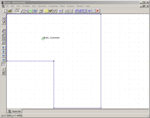
Figure 2: Completed example in the preprocessor.
2.1 Create model
Start FEMM by selecting the "FEMM 4.2" entry placed in the "FEMM 4.2" section of your start menu. After the program starts, select "File|New" from the main menu. A dialog will appear allowing you to select the type of problem to be created. Select "Heat Flow Problem" from the drop list for the current example. A blank problem will appear.
Select
“nodes” from the tool bar (this is the farthest button on the left with a small
black box: ![]() )
and place 6 nodes for the corner of a box (at, for example, (0,1), (1,1), (1,0)
,(2,0),(2,2) and (0,2)). One can place
nodes either by moving the mouse pointer to the desired location and pressing
the left mouse button, or by pressing the <TAB> key and manually entering
the point coordinates via a popup dialog.
)
and place 6 nodes for the corner of a box (at, for example, (0,1), (1,1), (1,0)
,(2,0),(2,2) and (0,2)). One can place
nodes either by moving the mouse pointer to the desired location and pressing
the left mouse button, or by pressing the <TAB> key and manually entering
the point coordinates via a popup dialog.
Select
“lines” from the tool bar (second button from the left with a blue line: ![]() ).
To select a node to be the endpoint of a line, click near each desired endpoint
with the left mouse button. Select connect the points as pictured in Figure 2
using this mouse endpoint selection approach.
).
To select a node to be the endpoint of a line, click near each desired endpoint
with the left mouse button. Select connect the points as pictured in Figure 2
using this mouse endpoint selection approach.
2.2 Add materials to the model
Select “Properties|Materials Library” off of the main menu. A dialog will appear that will allow you to drag materials from the library into your model. In the library, open up the "Nonmetallic Solids" folder, then the "Bricks" folder inside it. Drag the "Brick, Common" entry from the library into your model. Press the “OK” button to exit the materials library.
2.3 Define materials for each region
Now click
on “Block Labels” (the tool bar button with green circles ![]() ),
and place a block label in the middle of the solution domain, between the inner
and outer squares. Like node points, block labels can be placed either by a
click on the left mouse button, or via the <TAB> dialog.
),
and place a block label in the middle of the solution domain, between the inner
and outer squares. Like node points, block labels can be placed either by a
click on the left mouse button, or via the <TAB> dialog.
Right click on the block label node for the outer box so that the node turns red, denoting that it is selected. Press space to “open” the selected block label. A dialog will pop up containing the properties assigned to the selected label. Set the “Block type” to “Brick, Common”. Uncheck the “Let Triangle choose Mesh Size” checkbox and enter “0.05” for the “Mesh size”. The mesh size parameter defines a constraint on the largest possible elements size allowed in the associated section. The mesh generator attempts to fill the region with nearly equilateral triangles in which the sides are approximately the same length as the specified “Mesh size” parameter. When the “Let Triangle choose Mesh Size” box is checked, the mesh generator is free to pick its own element size, usually resulting in a somewhat coarse mesh.
2.4 Define Boundary Conditions
Select “Properties|Boundary” from the menu bar, then click on the "Add Property" button. Replace the name “New Boundary” with “Inner Boundary”. Select the "Convection" entry from the "BC Type" block list. For the inner surface of the chimney, we will assume that the air temperature inside the chimney is 800K and that the heat transfer coefficient is 10 W/m*K. Enter these values into the appropriate active edit boxes. Hit “OK”. You have just defined a convection boundary condition for the inner surface of the chimney, but you have yet to assign this boundary condition to a particular part of the model.
Repeat the above process, but instead name the new boundary condition “Outer Boundary” and apply a heat transfer coefficient of 5 W/m*K and a temperature of 300K.
Select “lines” from the toolbar then right click on the each of the two segments belonging to the inner chimney surface. When a segment turns red, you have selected it. Now press space bar and the “Segment Properties” window will appear. From the “Boundary Property” drop list change the selection from “<None>” to “Inner Boundary”. Repeat this process for the outer boundary, but set the boundary type to “Outer Boundary”.
2.5 Set Problem Characteristics
Select “Problem” from the menu bar. In the dialog that appears, make sure the problem type is “planar”. Set the length units to “Meters” and set the “depth” parameter to 20. The default solver precision of 10-8 (i.e. solution determined to single precision accuracy) generally need not be modified. If desired, a descriptive commend can be added in the “Comment” edit box.
2.6 Generate Mesh and Run FEA
Now save
the file and click on the toolbar button with yellow mesh: ![]() .
This action generates a triangular mesh for your problem. If the mesh spacing
seems to fine or too coarse you can select block labels or line segments and
adjust the mesh size defined in the properties of each object. When you are satisfied with the mesh, click
on the “turn the crank” button
.
This action generates a triangular mesh for your problem. If the mesh spacing
seems to fine or too coarse you can select block labels or line segments and
adjust the mesh size defined in the properties of each object. When you are satisfied with the mesh, click
on the “turn the crank” button ![]() to run the FEA algorithm over your model.
to run the FEA algorithm over your model.
Processing status information will be displayed in a dialog box while the solver runs. If the progress bars do not seem to be moving then you should probably cancel the calculation. This can occur if insufficient boundary conditions have been specified. For this particular problem, the calculations should be completed in less than a second (although the solution time is highly dependent on the speed of the machine running the analysis). There is no confirmation for when the calculations are completed, the status window just disappears when the processing is finished.
2.7 Display Results
Click on
the glasses icon ![]() to open the solution in a postprocessor
window. The solution will then be displayed, as pictured in Figure 3. By default, a color density plot of voltage
is displayed when the postprocessor starts.
If desired, the default behaviors can be changed via the Edit|Preferences
selection on the main menu of both the preprocessor and postprocessor.
to open the solution in a postprocessor
window. The solution will then be displayed, as pictured in Figure 3. By default, a color density plot of voltage
is displayed when the postprocessor starts.
If desired, the default behaviors can be changed via the Edit|Preferences
selection on the main menu of both the preprocessor and postprocessor.
The heat
flux through the chimney can then be determined using the integration
capabilities of FEMM. First, push the ![]() button to put the postprocessor into Contour
mode. In this mode, contours through
the geometry can be defined for the purposes of computing line integrals or for plotting.
button to put the postprocessor into Contour
mode. In this mode, contours through
the geometry can be defined for the purposes of computing line integrals or for plotting.
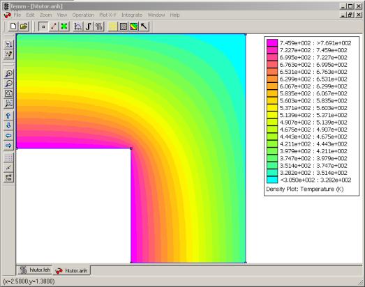
Figure 3: Solution to the example rendered in the postprocessor.
Create a contour that goes through the center of the chimney for the purposes
of computation. Either with the mouse
or with the <TAB> key dialog, add the points (0,1.5), (1.5,1.5), and
(1.5,0) to the contour. Press the ![]() button to evaluate the flux passing normal to
the defined contour. In the dialog that
pops up, select "Heat Flux (F.n)" as the integral type and press
"OK". The integral result
will then appear, which should be about 14883.6W if the problem was been
correctly constructed. To obtain the
result for the entire chimney, the result would be multiplied by four, yielding
59534.4W as the total heat flow.
button to evaluate the flux passing normal to
the defined contour. In the dialog that
pops up, select "Heat Flux (F.n)" as the integral type and press
"OK". The integral result
will then appear, which should be about 14883.6W if the problem was been
correctly constructed. To obtain the
result for the entire chimney, the result would be multiplied by four, yielding
59534.4W as the total heat flow.
4. Conclusions
From this basic introduction you should have gained the following principles:
- How to create your model space using nodes and lines.
- How to add material types to your model and how to assign them to regions.
- How to specify the finite element mesh size.
- How to define boundary conditions for your model.
- How to apply boundary conditions to line segments in the model.
- How to run the mesh generator and solver.
- How to run the postprocessor and compute the resulting heat flux.
A completed version of this example problem is available as htutor.feh, included in the FEMM binary distribution.
The same problem can also be implemented via scripting either in Lua (which is built into FEMM), Matlab/Octave (using a library of FEMM-related Matlab/Octave commands that are part of the regular FEMM distribution), or Matlab (using the MathFEMM package, which is also included in the regular FEMM distribution). Scripting examples of this same tutorial problem are included in the distribution. The Matlab/Octave and Mathematica versions are included in the distribution as htutor.m and htutor.nb, respectively. A Lua version of the script is included below in the Appendix. These scripting examples implement all of the above steps in a programmatic way.
The finite element solution to a fairly simple problem in heat conduction been presented in a step-by-step fashion. Hopefully, this example will allow you to apply the program to practical problems with more complicated geometries.
Appendix: Lua Script version of Heat Flow Tutorial Problem
--
-- Heat Flow Scripting Example
--
-- David Meeker
-- dmeeker@ieee.org
-- March 1, 2005
--
-------------------------------------------------------
newdocument(2);
-- define problem parameters
hi_probdef("meters","planar",1e-8,20,30);
-- add in materials and boundary conditions
hi_addmaterial("Brick",0.7,0.7,0);
hi_addboundprop("Outer Boundary",2,0,0,300,5,0);
hi_addboundprop("Inner Boundary",2,0,0,800,10,0);
-- draw the geometry
hi_addnode(0,1);
hi_addnode(0,2);
hi_addnode(2,2);
hi_addnode(2,0);
hi_addnode(1,0);
hi_addnode(1,1);
hi_addsegment(0,1,0,2);
hi_addsegment(0,2,2,2);
hi_addsegment(2,2,2,0);
hi_addsegment(2,0,1,0);
hi_addsegment(1,0,1,1);
hi_addsegment(1,1,0,1);
hi_addblocklabel(1.5,1.5);
-- apply the defined matrial to a block label
hi_selectlabel(1.5,1.5);
hi_setblockprop("Brick",0,0.05,0);
hi_clearselected()
hi_zoomnatural()
-- apply the boundary conditions
hi_selectsegment(1,0.5);
hi_selectsegment(0.5,1);
hi_setsegmentprop("Inner Boundary",0,1,0,0,"<None>");
hi_clearselected()
hi_selectsegment(2,0.5);
hi_selectsegment(0.5,2);
hi_setsegmentprop("Outer Boundary",0,1,0,0,"<None>");
hi_clearselected()
-- the file has to be saved before it can be analyzed.
hi_saveas("c:/progra~1/femm42/examples/lua-htutor.feh");
hi_analyze()
-- view the results
hi_loadsolution()
-- we desire to obtain the heat flux, just like in the
-- tutorial example. first, define an integration contour
ho_seteditmode("contour");
ho_addcontour(0,1.5);
ho_addcontour(1.5,1.5);
ho_addcontour(1.5,0);
heatflux,avgheatflux=ho_lineintegral(1);
result=format('The total heat flux is %f',4*heatflux);
-- there are multiple ways to report results. The results could
-- be printed to the Lua console via:
showconsole();
print(result);
-- and/or reported to the user in a message box with:
messagebox(result);