Induction Motor Example
David Meeker
August 20, 2004
Introduction
A frequently asked question about FEMM is “how do you analyze an induction motor?” Generally, one would like to use the program to model the performance of an induction machine at speed and under load. Currently, however, all analyses in FEMM are of mechanically static configurations. Rather than modeling the machine’s behavior directly, one must infer the performance at speed and load through a series of simulations of static configurations.
An induction machine with a moving rotor with can be modeled using a relatively simple circuit model. The purpose of the static FEMM analyses is then to identify the parameters in the circuit model. This circuit model can then be used under a wide variety of conditions (e.g. even transient simulations). Although circuit parameters can often be approximated by closed-form expressions in explicit terms of the motor geometry, the point of identifying these parameters via finite element analyses is to validate the approximations and simplifications that inevitably must be made in the derivation of the analytical design formulas.
The purpose of this example is to demonstrate, in a relatively step-by-step manner, how one goes about building and identifying an induction machine model using FEMM. This example will specifically consider a 220V, 50 Hz, 2 HP motor.
The files referred to in this article are available here.
Induction Motor Model
A reasonable model of an induction motor must first be identified before the parameters in that model can be deduced. A reasonable model to assume might be the one pictured in Figure 1. This model is meant to represent one phase of an induction machine operating in steady state (i.e. at a constant electrical frequency and a constant mechanical speed). In this model, all leakage is lumped on the stator side of the circuit in inductance Ll. The coupling to the rotor and the currents on the rotor are represented by parallel paths through the inductor, M, representing the inductance of the magnetic circuit linking the rotor and stator and through resistor Rr, representing work dissipated as heat in the rotor and delivered to the load as mechanical power. In this circuit equation, v represents the phase voltage, the RMS voltage applied across each phase of the machine, and i represents the phase current, the RMS current through each phase of the machine. These are important distinctions, because depending on how the motor is wired (i.e. wye or delta wiring), line-to- line voltage may or may not be equal to phase voltage, and line current may or may not be equal to phase current. To remove any ambiguity, this note will deal with a model represented exclusively in terms of phase current and phase voltage.
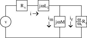
Figure 1: Simple steady-state per-phase induction motor model.
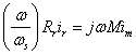
The symbol ω represents the applied electrical frequency (in radians/second). The symbol ωs represents the difference between the rotor’s mechanical frequency and its electrical frequency. If the stator is constructed with p pole pairs, we can define slip frequency ωs in terms of electrical frequency and mechanical rotor speed ωr as:
![]()
Now that we have a model of the motor, we can use this model to derive some useful relationships between phase current, phase voltage, and torque.
Motor Impedance
The impedances of the motor can be added together in the same fashion as resistors, using the same rules for parallel and series configurations. In case, the total impedance of the motor could be represented by Z, where:
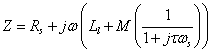
where τ is the rotor time constant, M/Rr.
The voltage is then related to the current via:
![]()
Per-Phase Flux Linkage
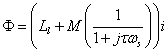
A result that will be useful later on in the note is the flux linkage of any particular phase. One can note that the second term in the impedance is multiplied by jω, which implies that this is a voltage contribution that has to do with the variation of flux at frequency ω. We can then imply that the flux, Φ, linking any phase is:
Dividing by current, we can obtain a slip frequency-dependent inductance. This result can be separated into real and complex components as:
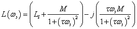 (1)
(1)
The dependency of this inductance on slip frequency provides us with a mechanism that we will later use to identify motor parameters. Since flux linkage is easy to calculate and can be obtained with high accuracy in the FEMM implementation, one can then use calculations of flux linkage at different slip frequencies to compare to (1) to identify the M, Ll, and Rr parameters of the motor.
Torque as a Function of Current
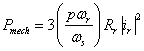
Since the example is a motor, one is ultimately concerned with generating torque. Torque can be implied directly from the circuit model. Consider, referring to Figure 1, the power that is dissipated in the rotor’s apparent “resistance”:
The multiplication by three is because this is a three-phase machine, and we are interested in the total rotor power in the machine. It is also assumed that ir is an RMS current. The rotor power can be decomposed into two separate losses: the resistive losses in the rotor, and the mechanical power delivered:
where the first term represents mechanical power and the second represents rotor losses. If we re-write the numerator of the mechanical power in terms of the mechanical speed (using the previous definition of slip frequency), we get:
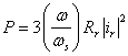
Lastly, noting that mechanical power is the product of torque and mechanical speed, we simply divide by ωr to get torque T:
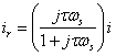
Although this is a perfectly valid expression for torque, it is in terms of rotor current rather than phase current. With a few more steps, the torque result can be written in terms of phase current. The voltage loop equation around the rotor is:
solving for rotor current, we get:
![]()
if we note that the total current is the sum of the magnetizing and rotor currents:
![]()
we can solve to obtain:
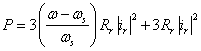
Taking the magnitude of ir and substituting into the torque expression yields:
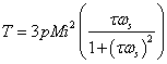
If current is held constant and slip frequency is varied, the curve shown in Figure 2 is obtained. The peak torque occurs at τωs=1.
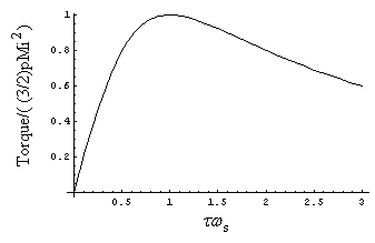
Figure 2: Constant current slip curve.
Now, once the parameters for the motor are determined, we can infer the force on the machine from those parameters and the operating conditions (current and slip frequency).
Identification of Model Parameters via Finite Element Analysis
The formulas developed above can be used as the basis for a finite element identification of motor parameters. Using FEMM, the rotor does not move; however, this presents no particular problem as far as parameter identification. In the zero speed case, slip frequency simply degenerates to ωs = &omega.
Analysis Approach
Based on the above there are at least two alternative approaches that could be followed. Perhaps the most obvious method would be to base parameter identification on torque results analyzed using a constant stator current over a range of frequencies.
Alternatively, one could attempt to fit against inductance results. Internally, the program obtains flux linkage by performing a volume integral that is closely related to the computation stored energy, a quantity which FEMM calculates with high accuracy. Results of this calculation are therefore expected to be more accurate than torque calculations. For this reason, a fit to inductance will be considered in this article.
The approach is then:
- To formulate a finite element model of the motor of interest
- Apply 3-phase currents to the stator windings model over a range of frequencies. (There is no need to worry about the values of rotor currents—the program computes them itself because the rotor currents are induced eddy currents)
- For each analysis, evaluate the flux linkage of one phase to get the information that is required to fit the parameters in the circuit model.
- Perform a regression analysis to get the parameter values.
Each of these steps will now described in detail, using a particular motor geometry as an example.
Finite Element Model Formulation
The particular motor of interest is intended to be a 2 HP motor running on a 220 Vrms line-to-line, 50 Hz, 3-phase supply. This motor is a 4-pole machine (i.e. p = 2) , implying that it will be running at slightly less than 1500 RPM. The winding configuration for one pole of the machine is pictured below in Figure 3. There are a total of 36 slots on the stator and 28 slots on the rotor. A total of 44 turns sit inside each slot (i.e. so that a phase current of 1 A would place a total of 44 Amp*Turns in a slot). The rotor’s diameter is 80 mm, and the clearance between the rotor and stator is 0.375 mm. The length of the machine in the into-the-page direction is 100 mm. Detailed dimensions on other aspects of the machine can be gleaned from the CAD file, 2horse.dxf.
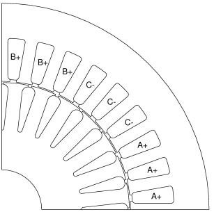
Figure 3: Example induction motor winding configuration.
This motor is intended to have the phases connected in a delta configuration. In the delta configuration, the phase voltage amplitude is equal to the line-to-line voltage amplitude, but the phase current amplitude is equal to 1/sqrt(3) of the line current amplitude (i.e. the phase current amplitude is roughly 60% of the line current amplitude).
The model of this geometry is contained in the input file, 2horse.fem. There are a number of important issues with respect to this geometry:
- Due to
symmetry considerations, only ¼ of the machine need be modeled. To make a valid ¼ model, anti-periodic
boundary conditions are used to link the edge at
 to the edge at θ=90o. Each anti-periodic boundary condition
can only be used to link one pair of segments. Since there are four pairs of segments to be linked, four
anti-periodic boundary conditions must be defined.
to the edge at θ=90o. Each anti-periodic boundary condition
can only be used to link one pair of segments. Since there are four pairs of segments to be linked, four
anti-periodic boundary conditions must be defined.
- Only linear materials are employed in the model. The above approach assumes that impedance is not a function of current amplitude, i.e. assuming linear materials. It should be noted that although the assumption of linear materials is adequate for many induction motor models, linear materials cannot be used to model machines with closed rotor slot geometries, because these machines rely on saturation in the thing section between slots to limit leakage flux to tenable levels. If this saturation is not modeled, nonphysical results are produced for the closed-slot geometry. Although FEMM can model nonlinear time-harmonic problems and is suitable for the analysis of closed-slot machines, the analysis approach is a bit different than is described in this note.
- For the present identification purposes, the stator iron is assumed to have a zero electrical conductivity (i.e. eddy currents in the iron are neglected.)
- The rotor bars are modeled as a grade of aluminum with a conductivity of 34.45 MS/m. This is consistent with 1100 aluminum at room temperature. Later, this resistance could be adjusted for the actual operating temperature by assuming that the resistance scales proportionally with the resistance of the aluminum.
The lua script, 2horse.lua, can now be run to evaluate the inductance of one of the phases in the motor versus slip frequency. The inductance is fairly simple to evaluate. The mo_getcircuitproperties command returns the flux linkage of the specified phase. Inductance can be obtained by dividing flux linkage by the phase current.
|
Frequency, Hz |
Real Inductance |
Imaginary Inductance |
|
0.25 |
0.3113897 |
-0.078562 |
|
0.5 |
0.2644535 |
-0.130207 |
|
0.75 |
0.2126343 |
-0.15379 |
|
1 |
0.1683203 |
-0.158362 |
|
1.25 |
0.1342043 |
-0.15323 |
|
1.5 |
0.1088912 |
-0.144139 |
|
1.75 |
0.0902097 |
-0.13398 |
|
2 |
0.076302 |
-0.124052 |
|
2.25 |
0.0657982 |
-0.114864 |
|
2.5 |
0.057736 |
-0.106568 |
|
2.75 |
0.0514475 |
-0.099154 |
|
3 |
0.0464669 |
-0.092553 |
Table 1: Inductance results from lua script.
Regression of Motor Parameters from Inductance Results
The regression of parameters from the inductance results can be posed as a linear parameter fitting problem. First, one can consider the imaginary part of the inductance results:
If we define:
![]()
we can re-arrange to get:
![]()
This equation is linear in the parameters c1 and c2. At each row in Table, &omegas and Li are specified, forming a total of 12 equations (because we evaluated the results at 12 frequencies) for the two unknowns. A least-squares fit is then used to pick the values of the coefficients that best satisfy all 12 equations.
To do the least-squares fit, build a matrix m and vector b:

where ωs,k and Li,k represent the kth data points for slip frequency and the imaginary inductance component. Also note that the slip frequency must be converted into radians per second for the units to come out right (i.e. multiply the frequency in Hz by 2π). The problem to be solved can then be represented by the matrix equations:

The least-squares solution is to this over-determined problem is:
Note that since the matrix to be inverted is only a 2-by-2 matrix, no “heavy lifting” is required to solve this problem.
For the example, the results are c1 = 0.0522906 and c2 = 0.0271847. From the definitions of c1 and c2 we can then imply that:
M = 0.317148 H
τ = 0.164878 sec.
A plot of the fit of the imaginary part of the inductance is shown in Figure 4. The fit is very good, implying that the simple model that we have assumed for the induction machine is OK for the present purposes.
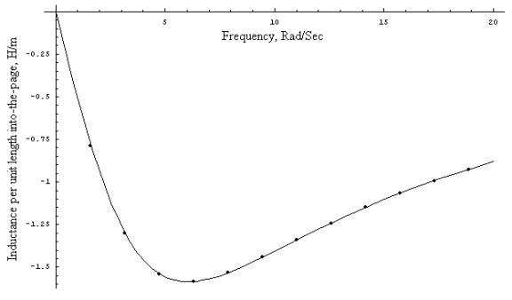
Figure 4: Fit of imaginary inductance curve to finite element “data points”.
The leakage inductance can be determined via a similar method using the real portion of the inductance. The real portion of the inductance is:
However, we now have values for τ and M as well as ωs and Lr. We can do the same sort of least-squares fit to identify leakage inductance Ll. However, this time, the best-fit Ll is just the average of the Ll that would be implied by each data point through:
In this case, the result is Ll = 0.0158 H.
Alternatively, one could perform a nonlinear optimization to directly minimizes the error in all equations simultaneously. If this is done, results are obtained that are similar to the above two-step approach.
M = 0.316428 H
<τ= 0.165258 sec
Ll= 0.0162968 H
Both approaches to regressing the parameters are shown in the Mathematica notebook, fit.nb
Comparison of Torque from Stress Tensor and Circuit Model
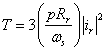
Above, we had derived the expression for torque:

where i is RMS phase current. If our model is any good, we ought to be able to compare the torque predictions to “measurements” of torque on the rotor computed via the weighted stress tensor block integral. To make this comparison, torque was evaluated via the stress tensor for a 1 Apk current at a number of different slip frequencies. The torque was then calculated using the motor parameters derived via the nonlinear fit method.
A comparison between the torque predicted from the circuit model and the results from the stress tensor is shown below in Figure 6. The agreement is very good in this case.
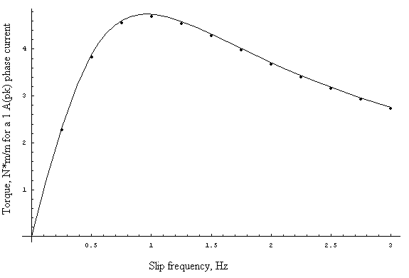
Figure 6: Comparison between stress tensor and circuit model force predictions.
Determination of Operating Point
In the previous section, we identified some parameters that can be used in the circuit equation of Figure 1. However, one can’t simply dump the numbers that have been identified from the 2D finite element model into the equation and expect them to provide a good match to experimental measurements of an actual motor. Several factors are at play:
- Increase in rotor resistance due to increase in temperature. Typically, resistive losses will heat the rotor to a temperature that is substantially higher than room temperature. The increase in resistivity of aluminum is about 40% for every 100C. The nominal operating temperature might be, for example, 80C, which would be a 24% increase in resistance. Typically, it is OK to simply scale the rotor resistance determined from finite element analysis using room temperature properties with resistivity. However, finding the actual operating temperature can imply the solution to thermal problem (which is coupled to the electrical design problem). We should note that this has the potential to be complicated—for our purposes, we will just assume a temperature as a reasonable operating point.
- Increase in rotor resistance due to end bars. The electric circuits on the rotor must be completed in the bars and the ends of the rotor. This part of the electric circuit path can substantially increase resistance, especially in machines that are short in the axial direction. If the geometry of these end bars is known, one can usually calculate the current that must be carried in any given section of the end bars. From the implied losses, one can adjust the rotor resistance to take account of this additional length in the circuit path.
- Flux leakage off of the rotor ends. The end bars also cause some additional flux leakage off the ends of the machine. This can be quite difficult to calculate—sometimes people will make specialized 2D finite element analyses of the ends in an attempt to get an estimate of these losses. This leakage is problematic, because it influences the relationship between current and force that would be inferred from the 2D finite element analysis. When one recasts the problem into the form of the circuit in Figure 1 (in which all of the leakage is lumped on the stator side), the rotor leakage makes the mutual inductance M appear to be smaller and the stator leakage Ll appear to be larger.
- Flux leakage off of the stator end turns. There is an analogous effect with the end turns of the stator windings. Some additional flux leakage results from flux that links the end turns through flux paths that are not included in the 2D model. This leakage does not affect the relationships between current and force that would be implied by a 2D finite element model. However, this leakage implies that more voltage will be required to obtain a given current at a given frequency.
- Core Losses. A significant amount of power is dissipated as core losses due to eddy currents and hysteresis in the iron. If we were being more complete, a decent model of these losses could be included by placing an extra resistor in parallel with the mutual inductance, M, to represent eddy current losses. Hysteresis losses can be represented via a complex-valued M. The hysteresis losses are then related to the complex part of M:
![]()
The correct eddy current resistor and imaginary part for M can be determined by an extended version of the impedance fitting approach that has been presented.
- Windage and Friction Losses. These are mechanical losses that also show up as additional power that must ultimately come out of the terminals.
Often, one has a specified terminal voltage, and one would like to determine the mechanical speed, stator current, efficiency, etc., that are associated with supporting a specific mechanical output. To get a realistic estimate of these quantities, the above non-idealities must be taken into account.
The companion Mathcad 7 worksheet operatingpoint.mcd is intended to show how one might take some of these issues into account to determine and operating point, in combination with the results derived from the finite element parameter identification.
Conclusions
In general, there is a lot of subtlety involved in the design and modeling of induction machines. This present document only scratches the surface of induction motor modeling. Among the issues that have been neglected in the current analysis are:
- A design feature that is common in induction motor design but not addressed in the present analysis is rotor skew. The reason for this skew is so that the rotor bars see flux linkage that has less harmonic content.
- Harmonic effects are neglected in motionless analysis. The higher harmonics can create forces (and losses) that are not anticipated by the simple model presented here.
- “Deep bar” rotors. To get better starting torque behavior, many induction motors are designed with more complicated (e.g. two layer) rotor bar topologies. These are not well-modeled by the circuit that has been presented here. A network of additional inductors and resistors on the rotor branch of the circuit is required to model these bars. A similar impedance-fitting approach could be used to identify values for impedances in such a network model.
- Nonlinear materials. Generally, induction motors are designed to run near saturation. Some induction motor designs have covered rotor slots (to reduce harmonic content of the flux in the gap) that must saturate so that leakage flux is not excessive.
The identification of induction model parameters from finite element analyses has not been neglected in the literature. A good example is:
D. Dolinar et al., “Calculation of two-axis induction motor model parameters using finite elements,” IEEE Transactions on Energy Conversion, 12(2):133-142, June 1997.
The full text of this paper is available via the web at:
The Dolinar paper also contains an excellent bibliography of the work of other authors in the area of identification of model parameters from finite element analyses.
Also see https://www.diva-portal.org/smash/get/diva2:790873/FULLTEXT01.pdf for a version of this example benchmarked against other software.
| File | Last modified | Size |
|---|---|---|
| imxfiles.zip | 2018-10-13 19:18 | 714Kb |