FEMM 4.2 Magnetostatic Tutorial
David Meeker
dmeeker@ieee.org
revised December 14, 2013
1. Introduction
Finite Element Method Magnetics (FEMM) is a finite element package for solving 2D planar and axisymmetric problems in low frequency magnetics and electrostatics. The current version of the program program runs under runs under Windows 2000, XP, Windows 7 and Windows 8. The program has also been tested running in Wine on Linux machines. The program can be obtained via the FEMM home page at https://www.femm.info.
The package is composed of an interactive shell encompassing graphical pre- and postprocessing; a mesh generator; and various solvers. A powerful scripting language, Lua 4.0, is integrated with the program. Lua allows users to create batch runs, describe geometries parametrically, perform optimizations, etc. Lua is also integrated into every edit box in the program so that formulas can be entered in lieu of numerical values, if desired. (Detailed information on Lua is available from http://www.lua.org/manual/4.0/) There is no hard limit on problem size—maximum problem size is limited by the amount of available memory. Users commonly perform simulations with as many as a million elements, though simulations with tens of thousands of elements are typical.
The purpose of this document is to present a step-by-step tutorial to help new users get "up and running" with FEMM. In this document, the solution for the field of an air-cored coil is considered. Although the objective of the tutorial is for the reader to build the model on their own, the completed tutorial.fem can also be downloaded.
2. Model Construction and Analysis
This will take you through a step-by-step process to analyze the magnetic field of an aircored solenoid sitting in open space. The coil to be analyzed is pictured in Figure 1. The coil has an inner diameter of 1 inch; an outer diameter of 3 inches; and an axial length of 2 inches. The coil is built out of 1000 turns of 18 AWG copper wire. For the purposes of this example, we will consider the case in which a steady current of 1 Amp is flowing through the wire.
In FEMM, one models a slice of the axisymmetric problem. By convention, the r=0 axis is understood to run vertically, and the problem domain is restricted to the region where r≥0. In this convention, positive-valued currents flow in the into-the-page direction.
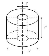
Figure 1: Air-cored coil to be analyzed in first example.
2.1 Create a New Model
Run the FEMM application by selecting femm 4.2 from the femm 4.2 section of the Start Menu. The default preferences will bring up a blank window with a minimal menu bar.
Select New from the main menu. A dialog will pop up with a drop list allowing you to select the type of new document to be created. Select the Magnetics Problem entry and hit the OK button. A new blank magnetics problem will be created, and a number of new toolbar buttons will appear.
2.2 Set Problem Definition
The first task is to tell the program what sort of problem is to be solved. To do this, select Problem from the main menu. The Problem Definition dialog will appear. Set Problem Type to Axisymmetric. Make sure that Length Units is set to Inches and that the Frequency is set to 0. When the proper values have been entered, hit the OK button.
2.3 Draw Coil
Switch Nodes mode by pressing the Operate on nodes toolbar button
 . Place nodes at (0.5,-1), (1.5,-1), (1.5,1) and (0.5,1) defining the extents of the coil. One can place nodes either by moving the mouse pointer to the desired location and pressing the left mouse button, or by pressing the <TAB> key and manually entering the point coordinates via a popup dialog.
 Select the Operate on segments toolbar button
 so that lines can be drawn connecting the points. By selecting the nodes defining the coil with left mouse button clicks in sequence, one obtains lines between each of the nodes and result in a large connected box.
 2.4 Place Block Labels
Now click on the Operate on Block Labels toolbar button denoted by concentric green circles
 . Place a block label in the coil region, and place one in the air outside the coil region. Like node points, block labels can be placed either by a click on the left mouse button, or via the <TAB> dialog. The program uses block labels to associate materials and other properties with various regions in the problem geometry. Next, we will defined some material properties, and then we will go back and associate them with particular block labels.
 NOTE: If snap-to-grid is enabled then it may be sometimes be difficult to place the block label in the empty space. If this is the case, disable snap-to-grid by de-selecting the tool bar button with the point and arrow.
2.5 Add materials to the model
Select Properties|Materials Library off of the main menu. The drag-and-drop Air from Library Materials to Model Materials to add it to the current model. Go into the Copper AWG Sizes folder and drag 18 AWG into Model Materials. Click on OK.
2.6 Add a "Circuit Property" for the coil
Select Properties|Circuits off of the main menu. On the dialog that appears, push the Add Property button to create a new circuit property. Name circuit by replacing the new circuit name with Coil. Specify that the circuit property is to be applied to a wound region by selecting the Series radio button. Enter 1 as the Circuit Current. The j edit box denotes the imaginary component of the current, which is used in time harmonic problems to denote the phase of the current. In this case, the problem is magnetostatic, so the imaginary component is ignored—just put zero in the j edit box. Click on OK for both the Circuit Property and Property Definition dialogs.
2.7 Associate properties with block labels
Right click on the block label node in the air region outside the coil. The block label will turn red, denoting that it is selected. Press <SPACE> to “open” the selected block label (Instead of pressing the space bar, one can use the Open up Properties Dialog toolbar button
 ). A dialog will pop up containing the properties assigned to the selected label. Set the Block type to Air. It usually sufficient to accept the default mesh density by checking the Let Triangle choose Mesh Size checkbox. If a finer mesh is desired, the box can be uncheck and a prescribed value entered into the Mesh size edit box. The mesh size parameter defines a constraint on the largest possible elements size allowed in the associated section. The mesher attempts to fill the region with nearly equilateral triangles in which the sides are approximately the same length as the specified Mesh size parameter. Click on OK. The block label will then be labeled as Air.
Select and open the block label node inside the coil region. However, set this Block type to Copper. We want to assign currents to flow in this region, so select the Coil circuit from the In Circuit drop list. The Number of turns edit box will become activated if a series-type circuit is selected for the region (e.g the Coil property that was previously defined). Enter 1000 as the number of turns for this region, denoting that the region if filled with 1000 turns wrapped in a counter-clockwise direction (i.e. positive turns in the right-hand-screw rule sense). Click on OK.
NOTE: If we wanted to denote that the turns are wrapped in a counter-clockwise direction instead, we could have specified the number of turns to be –1000.
2.8 Create Boundary Conditions
This example is an “open boundary” problem. That is, one would like to solve for the field of the coil in an unbounded space, unaffected by a nearby computational boundary. However, the finite element method always requires that problems be solved on a bounded domain. To approximate an unbounded domain, click on the Create IABC Open Boundary button
 on the toolbar. This button brings up the Open Boundary Builder wizard that create a boundary structure that accurately emulates the impedance of an unbounded domain. The wizard is shown below as Figure 2.
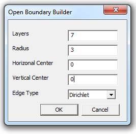
Figure 2: Open Boundary Builder wizard.
It is generally sufficient to simply accept the suggested boundary parameters by hitting OK. However, for the purposes of this problem, radius of 3 and a center of (0,0) was specified (by specifying parameters as shown in Figure 2).
The completed geometry looks as in Figure 3. The multi-layer structure is built automatically after OK is pressed on the Open Boundary Builder, and it provides all necessary boundary conditions for the problem.
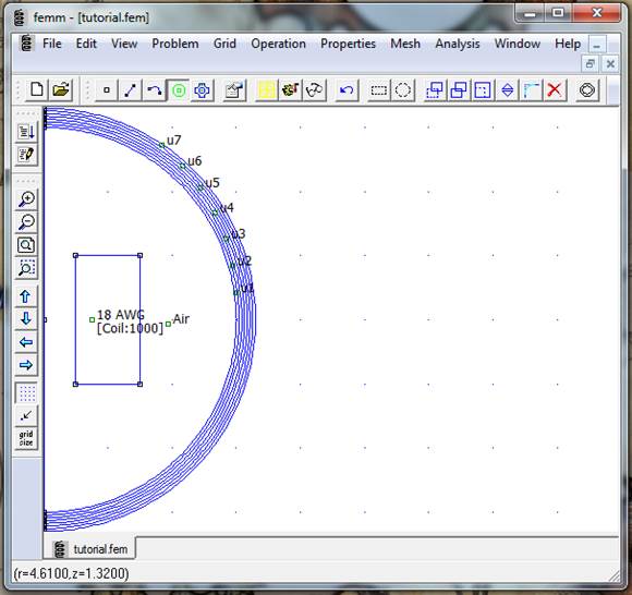
Figure 3: Completed coil model, ready to be analyzed.
2.9 Generate Mesh and Run FEA
Now save the file and click on the toolbar button with yellow mesh:
 . This action generates a triangular mesh for your problem. If the mesh spacing seems to fine or too coarse you can select block labels or line segments and adjust the Mesh size defined in the properties of each object. To adjust all of the mesh sizes in your model at once, press the <F3> button to refine the mesh in all blocks or the <F4> button to coarsen the mesh in all blocks. Once the mesh has been generated, click on the “turn the crank” button
  to analyze your model.
 Processing status information will be displayed. If the progress bars do not seem to be moving then you should probably cancel the calculation. This can occur if insufficient boundary conditions have been specified. For this particular problem, the calculations should be completed within a second. There is no confirmation for when the calculations are complete, the status window just disappears when the processing is finished.
3. Analysis Results
Click on the glasses icon
 to view the analysis results. A post-processor window will appear. The post-processor window will allow you to extract many different sorts of information from the solution.
 3.1 Point values
Just like the pre-processor, the post-processor window has a set of different editing modes: Point, Contour, and Area. The choice of mode is specified by the mode toolbar buttons, i.e.
 where the first button corresponds to Point mode, the second to Contour mode, and the third to Area mode. By default, when the program is first installed, the post-processor starts out in Point mode. By clicking on any point with the left mouse button, the various field properties associated with that point are displayed in the floating FEMM Output window. Similar to drawing points in the pre-processor, the location of a point can be precisely specified by pressing the <TAB> button and entering the coordinates of the desired point in the dialog that pops up. For example, if the point (0,0) is specified in the pop-up dialog, the resulting properties displayed in the output window are as pictured in Figure 4.
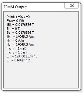
Figure 4: Display of field values at the point (0,0).
3.2 Coil terminal properties
With FEMM, it is straightforward to determine the inductance and resistance of the coil as seen from the coil's terminals. Press the
 button to display the resulting attributes of each Circuit Property that has been defined. For the Coil property defined in this example, the resulting dialog is pictured in Figure 5.
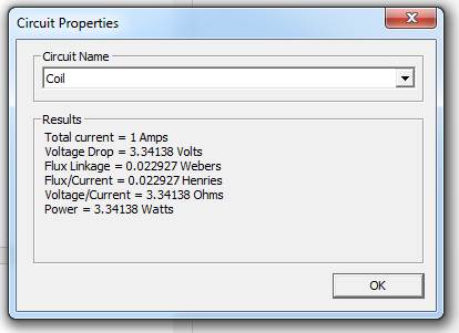
Figure 5: Circuit Property results dialog.
Since the problem is linear and there is only one current, the Flux/Current result can be unambiguously interpreted as the coil's inductance (i.e. 22.9 mH). The resistance of the coil is the Voltage/Current result (i.e. 3.34 Ω).
3.3 Plotting field values along a contour
FEMM can also plot values of the field along a user-defined contour. Here, we will plot the flux density along the centerline of the coil. Switch to Contour mode by pressing the Contour Mode toolbar button. You can now define a contour along which flux will be plotted. There are three ways to add points to a contour:
1. Left Mouse Button Click adds the nearest input node to the contour;
2. Right Mouse Button Click adds the current mouse pointer position to the contour;
3. <TAB> Key displays a point entry dialog that allows you to enter in the coordinates of a point to be added to the contour.
Here, method 1 can be used. Click near the node points at (0,4), (0,0), and (0,-4) with the left mouse button, adding the points in the above order. Then, press the Plot toolbar button
 . Hit OK in the X-Y Plot of Field Values pop-up dialog (as shown in Figure 6). The default selection is magnitude of flux density. If desired, different types of plot can be selected from the drop list on this dialog.
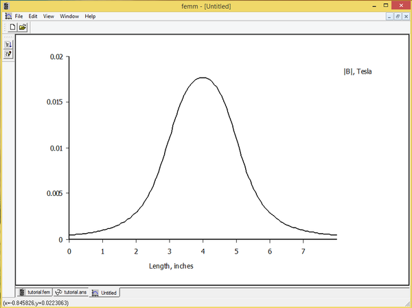
Figure 6: Plot of flux density along the axis of the coil.
NOTE: It is often the case in the solution to magnetic problems that the field values are discontinuous across a boundary. In this case, FEMM determines which side of the boundary will be plotted based on the order in which points are added. For example, if points are added around a closed contour in a counterclockwise order, the plotted points will lie just to the inside of the contour. If the points are added in a clockwise order, the plotted points will lie just to the outside of the contour. The implication to our example problem is that the contour along the r=0 should be defined in order of decreasing z (i.e. counterclockwise so that the plotted points will lie inside the solution domain instead of outside it, where the field values are not defined).
3.4 Plotting Flux Density
By default, when the program is first installed, only a black-and-white graph of flux lines is displayed. Flux density can be plotted as a color density plot, if you so desire. To make a color density plot of flux, click on the rainbow-shaded toolbar button
 to generate a color flux density plot. When the dialog box comes up, select the Flux density plot radio button and accept the other default values. Click on OK. The resulting solution view will look similar to that pictured in Figure 7.
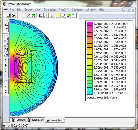
Figure 7: Color flux density plot of solution.
4. Conclusions
You have now completed your first model of a magnetic problem with FEMM. From this basic introduction, you have been exposed to the following concepts:
• How to draw a model using nodes, segments, arc, and block labels;
• How to add material to your model and how to assign them to regions;
• How to define a boundary for your model;
• How to analyze a problem;
• How to inspect local field values;
• How to plot field values along a line;
• How to compute inductance and resistance;
• How to display color flux density plots.
Hopefully, this tutorial has presented you with enough of the basics of FEMM so that you can explore more complicated problems without getting sidetracked by the mechanics of how a problem is drawn and analyzed.