Magnetic Circuit Derivation of Energy Stored in a Permanent Magnet
David Meeker
dmeeker@ieee.org
April 5, 2007
Introduction
The calculation of the energy stored in a permanent magnet is, perhaps surprisingly, something of a contentious topic. Contemporary works take multiple approaches to this issue [1] [2] [3]. The objective of this note is to derive a representation of stored energy in permanent magnets that is:
- Consistent with the stored energy calculated from a magnetic circuit model; and
- Consistent with the permanent magnet’s operating point in the second quadrant of its demagnetization curve.
A magnetic circuit-based approach to deriving stored energy provides an intuitive understanding of stored energy in permanent magnets. The resulting energy expression is also consistent with all granularities of analysis, from magnetic circuits to 3D finite elements calculations.
For simplicity of this note, only materials with linear 2nd quadrant demagnetization curves are considered. This assumption covers most grades of NdFeB and SmCo magnets. It is possible to extend the analysis to the case of materials with non-linear demagnetization curves (e.g. alnico magnets), but this generalization is not considered here.
Permanent Magnet Demagnetization Curve
To establish how a permanent magnet normally operates, the magnetization process of a permanent magnet from an initially demagnetized state can be considered. A generic magnetization curve for a permanent magnet is shown in Figure 1. The magnetization process can be tracked through four steps:
- The permanent magnet begins in an initially demagnetized state at field intensit H=0 and flux density B=0.
- The magnet is wrapped with a coil that supplies the field intensity needed to magnetize the permanent magnet material. As current in the coil wrapping the magnet material is increased, the flux density in the magnetic material increases until the magnet saturates.
- As the applied field intensity is removed, the flux density inside the permanent magnet material also decreases. Through hysteresis mechanisms, the magnet retains flux density Br when the applied field intensity is H=0.
- With the addition of an air gap and/or an external demagnetizing field intensity, the magnet ends up operating somewhere in the second quadrant of the demagnetization curve, where H is negative-valued and B is positive-valued. The slope of the magnetization curve in the second quadrant is μ. Permeability μ is typically very close to μo, the magnetic permeability of free space. The intersection of the demagnetization curve with B=0 occurs at H=-Hc, where Hc is known as the coercivity of the magnetic material.
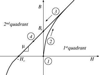
Figure 1: Magnetization curve for a permanent magnet.
The point of this explanation is to show the normal operating point of the magnet in the second quadrant and to explain how the magnet comes to be operating in this region. If a circuit model is to be valid for the purposes of energy computation, it should be able to model the magnet properly in its second quadrant operating point. The magnetic circuit should conform to the mathematical relationship between flux density, B,and field intensity, H, in the second quadrant:
|
|
Magnetic Circuit Representation of a Permanent Magnet
For the purposes of a circuit representation, the problem of a permanent magnet with highly permeable iron pole pieces can be considered. Such a geometry is pictured in Figure 2. In Figure 2, two iron pole pieces are attached to fashion the magnet into a horseshoe shape. The iron and magnet horseshoe is acting upon a thick iron wall. This problem is good for the purposes of considering energy stored the permanent magnet because all parts of the magnet are at more or less the same operating point.
Equation (1) relates the applied field to the flux at a single point, but because entire magnet is operating at the same B and H, eq. (1) can be used directly to imply a conservation of flux equation for the entire magnet. If a is the cross-section area of the magnet, the several magnet-related fluxes can be defined. The total flux flowing through the magnet, Φ, is defined as:
|
|
(2) |
The remanent flux in the magnet, Φr, is defined as:
|
|
(3) |
The demagnetizing flux in the magnet, Φd, is defined as:
|
|
(4) |
where the demagnetizing flux density is proportional to the demagnetizing field intensity:
|
|
(5) |
By multiplying both sides of (1) by area a and substituting the above magnet flux definitions, a flux conservation equation for the magnet is:
|
|
The magnetomotive force (MMF) drop over the magnet due to an external source is:
|
|
(7) |
The terms multiplied by the demagnetizing flux can be defined as the magnet's internal reluctance, Rm:
|
|
Let the combined reluctance of the flux return paths (mostly through the two air gaps between the magnet pole tips and the iron wall on the right side of Figure 2, but including the other return paths as well) be represented as load reluctance Rl.
Equation (6) implies a circuit with a flux source in parallel with a reluctance. The combined flux then flows through a load reluctance. The resulting magnetic circuit is pictured in Figure 3.
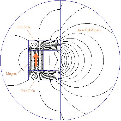
Figure 2: Permanent magnet with iron pole-pieces tugging on an iron wall.
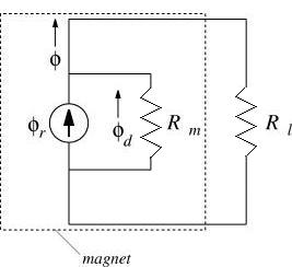
Figure 3: Circuit model of a permanent magnet driving a load reluctance.
Stored Energy Density in a Permanent Magnet
The advantage of the circuit representation with respect to the calculation of stored energy is that in the circuit representation, computation of stored energy is unambiguous. The energy stored in the magnet, Wm, is the energy stored in the magnet's internal reluctance:
|
|
Substituting for flux and reluctance yields:
|
|
(10) |
In can then be noted at a*l is the volume of the magnet. Since the example geometry has been selected so that the operating point is the same at every point in the magnet, the energy density, wm, in the magnet is then obtained as:
|
|
The energy result in eq. (11) is consistent with the stored energy expression presented in [1]. It is also possible to derive the same stored energy expression from a constant MMF source and series reluctance model of a permanent magnet, although the derivation is not as intuitive as that for a permanent magnet modeled as constant flux source and parallel reluctance. This derivation is discussed in Note 1.
It is also interesting to note that energy can be neither sourced nor sunk by the flux source in the magnet model. This result is derived below in Note 2.
Mechanical Work and Stored Energy
To evaluate the total energy stored in the permanent magnet and its surroundings, the flux through each reluctance in Figure 3 must first be obtained. For the circuit in Figure 3, one "node equation" and one "loop equation can be written:
|
|
(12) |
These equations can be solved for the unknowns Φ and Φr to obtain:
|
|
|
|
(14) |
The total energy can be obtained by summing up the energy for each reluctance:
|
|
By inspecting the total energy in (15), several interesting observations can be made.
- When the load reluctance, Rl, is zero, the magnetic field energy is zero. The load reluctance is zero (or close to it) when the magnet is clamped to the iron wall, eliminating the air gaps. This result is somewhat intuitively satisfying, since when the magnet is stuck to the iron wall, it can do no more work, because there is no further motion possible.
- When work is done on the magnet (e.g. moving it away from the wall), the stored energy increases. Again, this result is somewhat intuitively satisfying, because the mechanical work done on the magnet becomes stored energy in the magnetic field. This result is analogous to the weight*height potential energy that is gained by doing work against gravity, e.g. by lifting a mass off of the ground.
It can be shown (see [1]) that for a system with no coils (like the magnet in the present example), the force can be calculated directly from the change in magnetic field energy:
|
|
where x is a variable that denotes the position of the object upon which force is to be computed. Equation (16) is simply a mathematical way of expressing the idea that work done on the magnet gets stored in the PM's magnetic field. Torque in a system with no coils can also be calculated in a similar way:
|
|
(17) |
where θ represents an angular displacement rather than a linear one.
Computation of Coenergy
Coenergy is sort of a dual of stored energy that is often used to compute forces on systems with permanent magnets and current-carrying coils. Force and torque can be deduced by changes in energy with respect to position, but the process is complicated by the need to compute the energy that is sunk or sources by the supplies driving the coils over the change in position. Conversely, computing the change in coenergy for constant currents directly yields the mechanical work done on the system.[4]
The magnetic circuit representation does not give as much of an intuitive feel for coenergy as for energy. For the computation of coenergy, it is most expedient to go directly to the definition of coenergy in terms of B and H. Coenergy density (often denoted w’) is defined as [3]:
|
|
(18) |
If the desire is to obtain the correct change in coenergy with operating point, the choice of the lower bound of the integral, Ho, isn’t important as long as it is chosen consistently (i.e. so that it is a constant for a given material). The upper bound of the integral should be the operating point of interest.
For the purposes of coenergy computation, a convenient lower bound for the integral is Ho= -Hc. The coenergy density in the magnet (wm') is, for the case in which the flux density is aligned with the magnetization:
|
|
(19) |
This specific choice of Ho ensures that the coenergy density is never negative-valued. Noting the definition of magnet flux density B from (1) yields a simpler definition of coenergy inside the magnet:
|
|
(20) |
Graphical Interpretation of Stored Energy and Coenergy
It is now possible to interpret the stored energy and coenergy as regions mapped out on the demagnetization curve shown in Figure 1. This re-interpreted demagnetization curve is shown in Figure 4. A similar plot of energy and coenergy is presented in [5].
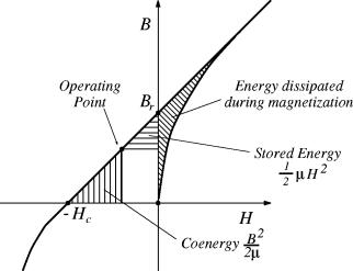
Figure 4: Demagnetization curve with graphical representation of energy.
As shown in the Figure, the area swept in the first quadrant represents the energy per unit volume (the integral of H(B) dB) that was needed to magnetize the material. This energy can never be recouped, even if a large field intensity is applied to the magnet to push its operating point back into the first quadrant, as shown in Figure 6. Pushing the magnet back into the first quadrant simply stores energy in the magnet without pulling out the energy associated with the magnet’s creation.
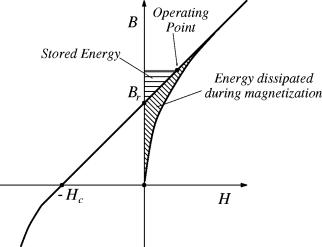
Figure 5: Permanent magnet with enough applied H to be operating in 1st quadrant.
Conclusions
This note has presented a magnetic circuit-based approach for deriving the energy stored in a permanent magnet. Through the use of a circuit representation, a better intuitive feel for the properties of a permanent magnet can be gleaned. This treatment explains the rationale for the permanent magnet stored energy and coenergy expressions implemented in the FEMM magnetics solver.
References
[1] H. Lovatt and P. Watterson, “Energy stored in permanent magnets,” IEEE Transactions on Magnetics, 35(1):505-507, Jan. 1999.
[2] P. Campbell, “Comments on ‘Energy stored in permanent magnets’,” IEEE Transactions on Magnetics, 36(1):401-403, Jan. 2000.
[3] J. Bastos and N. Sadowski, Electromagnetic Modeling by Finite Element Methods, CRC Press, 2003.
[4] G. Slemon, Electric Machines and Drives, Addison-Wesley, 1992.
[5] D. Dorrell, M. Popescu, and M. McGilp, “Torque Calculation in Finite Element Solutions of Electrical Machines by Consideration of Stored Energy,” IEEE Transactions on Magnetics, 42(10):3431-3433, Oct. 2006.
[6] “Thévenin's_theorem,” http://en.wikipedia.org/wiki/Thévenin's_theorem.
[7] “Norton’s theorem,” http://en.wikipedia.org/wiki/Norton's_theorem.
[8]V. Hnizdo, “Hidden Momentum and the Force on a Magnetic Dipole”, Magnetic and Electrical Separation, 3(4):259-265, 1992.
[9] H. A. Haus and J. R. Melcher, Electromagnetic Fields and Energy, online textbook.
Note 1: Thévenin circuit representation of a permanent magnet
Through the use of a Thévenin circuit representation [6], the constant flux source and parallel reluctance model of a permanent magnet of Figure 3 can be replaced by a constant magnetomotive force source in combination with a series reluctance. The Thévenin circuit representation of the circuit in Figure 3 is shown below in Figure 6.
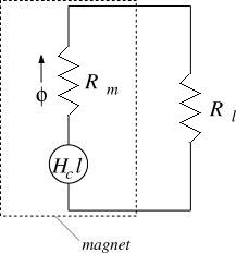
Figure 6: Thévenin magnetic circuit representation.
The Thévenin equivalent model produces exactly the same total flux through the magnet and exactly the same fluxes external to the magnet as compared to the flux source and parallel reluctance (Norton model [7]). The Thévenin model is widely used for the purposes of magnetic circuit calculation. It often reduces the number of loops in the circuit representation, simplifying the process of solving for flux.
However, the Thévenin model is not so intuitive for the purposes of computing the energy that the rest of the system stored in the magnet or receives from the magnet. The difficulty arises because the constant MMF source in the model can apparently source and sink power. The MMF source has to be taken into account in order to derive (9), the Norton model stored energy expression, from the Thévenin model.
To derive stored energy from the Thévenin model, it is easier to consider the circuit in Figure 7. An MMF source, i, provides a magnetizing/demagnetizing field that acts on the permanent magnet. In this case, the stored energy of the permanent magnet can be determined through conservation of energy—all magnetic energy that is sourced by i must be sunk by the magnet and vice versa. The relevant stored energy is not simply the energy stored in the magnet's internal reluctance, but rather the energy exchanged between the magnet and the rest of the system as the magnet's operating point changes.
A magnetic circuit equation for Figure 7 is:
|
|
For an easier comparison to previous stored energy results, it is useful to write the constant MMF, Hcl in terms of quantities used in the previous energy derviation.
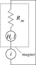
Figure 7: Circuit for computation of stored energy from a Thévenin model PM.
|
|
(22) |
Equation (21) can now be written as:
|
|
(23) |
Re-arranging to obtain i in terms of Φ yields:
|
|
(24) |
The energy sourced by i can be computed by considering an electric circuit that drives i. If resistance is negligible, the electric circuit equation associated with i is:
|
|
(25) |
where v is a voltage source that drives the electric circuit. The instantaneous power sourced by the circuit the product of voltage and current:
|
|
To obtain the total energy, power is integrated over time. Equation (26) can be used to write energy sourced by the coil, Wi, in terms of flux, rather than as an explicit function of time:
|
|
Equation (27) is the derived in a similar way in [4].
The energy calculated by (27) that is sourced by the coil must be the energy that is stored by the magnet, since there is no place else for the energy sourced by the coil to go. That is, Wi = Wm. The energy that the system stores in the magnet (or receives from the magnet, depending on the direction of change in Φ with time) is:
|
|
In (28), the bounds of integration for energy calculation have been select to be from the remanent flux condition (where i = 0), to the operating point of the magnet, Φ. By noting the definition of demagnetizing flux from (6), in (28) can be simplified to:
|
|
It can now be noted that the energy stored by the system in Thévenin magnet model in (29) is identical to the Norton model stored energy in (9), although internally, the Thévenin model behaves rather differently than the Norton model. The contortions in the derivation of energy stored are required because the Thévenin model apparently shifts the operating point of the magnet to the first quadrant—the magnet constant MMF model does not satisfy (1), the equation for the second quadrant demagnetization curve.
Note 2: Power sourced/sunk by a constant flux source.
An intuitive way of understanding why a constant flux source can neither source nor sink power is to follow an approach similar to that considered in Note 1. Consider a coil with negligible resistance that links a flux, Φ, driven by a voltage source, v. The circuit equation for the coil is:
|
|
The instantaneous power coming in and out of the voltage source is the product of the instantaneous coil current and coil voltage:
|
|
If there is no change in flux Φ with time, (31) shows that there is no power transferred to or from the coil.
A macroscopic physical realization of a constant flux source is a superconducting coil. A superconducting coil can be charged with current and the leads shorted together. The coil obeys (30), but since there is no external voltage source, v=0. The change in flux therefore must be zero, so the coil is a constant flux source. Although the flux is constant, the current in the coil changes to support the constant flux condition, e.g. if the coil is brought into the proximity of another superconducting coil, ferrous object, etc.
A reasonable schematic way of visualizing a permanent magnet material is a sparsely filled array of very small superconducting loops whose orientations are all fixed in the same direction. "Real" dipoles are made of circulating current rather than of magnetic charges. However, the circulating currents that make up these dipoles are not constant. The currents vary in a way similar to the currents in superconducting coils, satisfying conservation of momentum and conservation of energy. [8] [9]