Transient Loudspeaker Modeling
David Meeker
dmeeker@ieee.org
08Nov2015
Introduction
FEMM presently does not directly model the complete transient behavior of a loudspeaker. However, using a mapping of complex-valued inductance vs. frequency, as described at BlockedImpedance, parameters in a nonlinear transient model can be identified. This model should give reasonable results across a wide range of frequencies and signal levels.
This note will propose a frequency- and position-dependent inductance model and regress parameters that characterize the model from simulations of an example loudspeaker geometry. Then, the inductance model will be included in a complete system model of a loudspeaker operating in free air, using published Thiele/Small data as the basis for the loudspeaker's mechanical model.
It is worth noting that while the evaluated geometry is inspired by the pre-production prototype description of Bortot, the model should not be taken as representative of the production model. Any differences between production and prototype geometry are not reflected here, nor is the presence of any shorting rings incorporated in the production device reflected in the present model.
Inductance Model
Reference [1] describes several different frequency-dependent inductance models that have been used in the past. Here, we desire a model that is composed of discrete inductors and resistors like the LR-2 model. However, the LR-2 model doesn't have enough parameters to match the behavior of the finite element results from BlockedImpedance over a wide range of frequencies. A model with more resistors and inductors in the chain, however, can result in a good fit to finite element data. Testing various order models, a model with 5 inductors appears to be sufficient to represent the behavior of the BlockedImpedance system through the full evaluated frequency range. The circuit diagram of the higher order model is pictured in Figure 1. This form is commonly used in laminated devices like transformers [2] and magnetic bearings [3]. In those cases, it is possible to write analytical expressions for the L's and R's in the chain as functions of lamination geometry. In the case of loudspeakers, there is a similar small skin depth eddy current problem, so the same form is valid--however, it is hard to write analytical expressions for the parameters. Instead, they can be selected as a least-squares fit to finite element results.

Figure 1: Blocked Impedance model with L-R network representing the loudspeaker's frequency-dependent inductance.
Parameter Fitting
The circuit of Figure 1 can be realized as a set of circuit equations that can be derived by writing down an equation for each loop in the chain:
\[L(x) \frac{di}{dt} + R i = \left\{ \begin{matrix} v \\ 0 \\ \vdots \\ 0 \end{matrix} \right\} \]
where resistance matrix \(R\) and inductance matrix \(L\) are defined as:
\[ R = \left[ \begin{matrix} R_0 & & \\ & \ddots & \\ & & R_4 \end{matrix} \right] \]
\[ L = \left[ \begin{matrix} L_0 & -L_0 & 0 & 0 & 0 \\ -L_0 & L_0+L_1 & -L_1 & 0 & 0 \\ 0& -L_1& L_1+L_2& -L_2& 0 \\ 0& 0& -L_2& L_2+L_3& -L_3 \\ 0 & 0& 0& -L_3& L_3+L_4 \end{matrix} \right] \]
In this circuit, the \(i\) vector represents the current through the resistors in the network (e.g. \(i_0\) is the current through resistor \(R_0\) and so on). At each coil position, the L's and R's need to be identified to match the behavior of the finite element simulations, like that shown for the SSF-082 subwoofer shown in Figure 2.
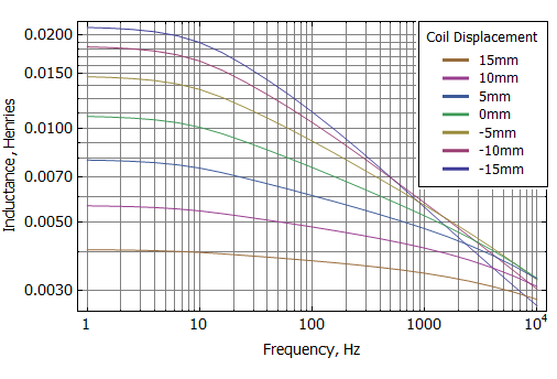
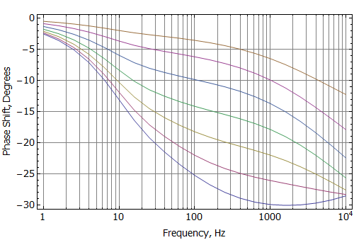
Figure 2: Blocked coil inductance vs. frequency at various coil offsets derived from finite element analysis.
Using the Mathematica or Matlab scripts at the bottom of the page, a least-squares fit can be used to determine the network inductances and resistances for each coil position. Then, a polynomial curve can be fit to the values for each parameter to interpolate the parameters across a range of positions. For the BlockedInductance SSF-082 example, the regressed inductances and resistances and their curve fits are shown in Figures 3 and 4.

Figure 3: Fit of network resistances to cubic curves.

Figure 4: Fit of network inductance to cubic curves.
The resulting parametric model, exercised across the entire range of coil positions, is shown in Figure 5. The network model with parameters that are a function of position provides a good reproduction of the FEA frequency-dependent inductance result across a wide range of positions and frequencies.

Figure 5: Complete parametric model (solid lines) vs FEA results (points) at various coil displacements.
Transient Model with Motion
The parametric model of blocked coil impedance can then be used as the basis for a dynamic model by including extra terms in the model that have to do with motion and by adding an equation that describes the mechanical system. The electrical equation, including motion terms, is:
\[L(x) \frac{di}{dt} + \left( \dot{x} \frac{dL(x)}{dx} + R \right) i = \left\{ \begin{matrix} v - \dot{x} Bl(x) \\ 0 \\ \vdots \\ 0 \end{matrix} \right\} \]
The Thiele/Small model for a loudspeaker in free space is essentially just at spring-mass-damper system driven by the force created by the current in the coil interacting with the magnetic field of the magnets and with the iron structure and induced eddy currents. The mechanical equation is:
\[ M_{ms} \ddot{x} + R_{ms} \dot{x} + \frac{1}{C_{ms}} x = \left\{ \begin{matrix} Bl(x) & 0 \ldots & 0 \end{matrix} \right\} \, i + \frac{1}{2} i' \frac{dL(x)}{dx}i \]
The \( \frac{1}{2} i' \frac{dL(x)}{dx}i \) terms is usually neglected from Thiele/Small analyses because it is a second-order term that is negligible for small \(i\). However, for accuracy of modeling possibly large currents and for a mathematical consistency with a position-dependent inductance matrix, this term is included in the present analysis. Note that by changing the mechanical equation, the effects of various cabinet configurations could be modeled.
These electrical and mechanical equations can be realized in a Simulink model, allowing the motion of the loudspeaker to be assessed for arbitrary input voltage waveforms. The Matlab/Simulink 2007b version simulation is below in the Files section. A picture of the Simulink model of a loudspeaker is shown below in Figure 6.

Figure 6: Complete loudspeaker model in Simulink.
The electrical equations and the expression for mechanical force on the coil are realized via an Embedded Matlab block (shown below), but the mechanical system is realized using regular Simulink blocks. It ought to be straightforward to implement the same model in Scilab/Xcos, but the Xcos version is not yet included here.
function [frc,didt] = EddySpeaker(x,dxdt,u,ie)
% Input units:
% x = Meters;
% dxdt = Meters/Second;
% u = Volts;
% ie = Amps;
% Output units;
% frc = Newtons;
% didt = Amps/Second;
% DC resistance at 20degC from FEMM
R0 = 5.76602;
% Parameters in inductance model derived from FEMM that tell how the inductands in and resistances
% in the eddy current model vary with position
lp=[0.011133411724445427,-0.0006909001256657835,7.07995364686979e-6,5.268050116280895e-7;
0.026567829297317415,0.00003710245831933369,0.000047795834393481296,2.3132117937500422e-6;
0.018672389734001454,0.00029966608330329284,0.0000131702675335866,2.878877822931358e-7;
0.008859866394875805,-1.508503789209484e-6,-2.10724331568106e-7,4.4373241308628945e-7;
0.002243047444369999,-0.00009450266905242674,-5.231332607562163e-7,5.961213280651767e-8];
rp=[3.5283284300296986,-0.02850093151777563,0.008376125777185784,0.0004513777632543519;
16.790766100941365,0.8084036166487055,0.07446972370380596,0.003254815058423787;
91.71944110105659,5.714371803005944,0.23158340989826123,0.00655093693193577;
345.68192863028486,10.432464583631907,0.5730951645736311,0.04282150212066517];
bp=[15.97658965332581, 0.005139750886155021, -0.039425839308130914,0.0000501469585189826];
% Compute the position-dependent values from the parameter matrices
mm=0.001;
xmm=x/mm;
X=[1;xmm;xmm^2;xmm^3];
dX=[0;1;2*xmm;3*xmm^2]/mm;
l=lp*X; % Position-dependent inductances
L0=l(1); L1=l(2); L2=l(3); L3=l(4); L4=l(5);
dl=lp*dX; % Derivative of indutances with respect to position
dL0=dl(1); dL1=dl(2); dL2=dl(3); dL3=dl(4); dL4=dl(5);
r=rp*X; % Position-dependent resistances
R1=r(1); R2=r(2); R3=r(3); R4=r(4);
Bl=bp*X; % Position-dependent Bl gain
Lmat=[L0, -L0, 0, 0, 0;
-L0, L0+L1, -L1, 0, 0;
0, -L1, L1+L2, -L2, 0;
0, 0, -L2, L2+L3, -L3;
0, 0, 0, -L3, L3+L4];
Rmat=[R0,0,0,0,0;
0,R1,0,0,0;
0,0,R2,0,0;
0,0,0,R3,0;
0,0,0,0,R4];
dLmat=[dL0, -dL0, 0, 0, 0;
-dL0, dL0+dL1, -dL1, 0, 0;
0, -dL1, dL1+dL2, -dL2, 0;
0, 0, -dL2, dL2+dL3, -dL3;
0, 0, 0, -dL3, dL3+dL4];
Uvec = [u - Bl*dxdt;0;0;0;0];
% Coumpute change in currents with respet to time;
didt = Lmat \ (Uvec - (Rmat + dxdt*dLmat)*ie);
% Compute force
frc=Bl*ie(1)+ (1/2)*ie'*dLmat*ie;
An example run, shown in Figure 7 below, shows the transient response of the model to a 120Hz, 1Vpk voltage applied to the terminals of the loudspeaker.

Figure 6: Complete loudspeaker model in Simulink.
Conclusions
Using FEMM's AC incremental solution functionality, the frequency- and position-dependent impedance of a loudspeaker can be identified. By selecting a suitable form, a parametric model that replicates the finite element results can be regressed. The parametric model can then be used in a transient model including various other nonlinear effects. In particular, Simulink can be used to integrate and view the transient loudspeaker model.
The model formulated in this note includes many nonlinear effects at work in loudspeakers, but there are still avenues for possible future improvement. Specifically, the program linearizes the results about a DC operating point established by the loudspeaker's permanent magnet. If the coil currents are big enough, the assumption of linearization about a DC operating point might not be a good one. In that case, there may be no recourse but nonlinear time-transient eddy current simulations with a coupled mechanical system model. The capability to do this sort of full time transient model is not yet included in FEMM, though such solutions are presently possible with some commercial solvers.
| File | Last modified | Size |
|---|---|---|
| SpeakerTransientModel.mdl | 2015-11-11 09:08 | 42Kb |
| ssf-082_vs_position_cont.nb | 2015-11-11 09:36 | 222Kb |
| ssf-082_vs_position_cont.pdf | 2015-11-11 09:37 | 265Kb |
| ssf-082_vs_position_cont_matlab.zip | 2015-11-11 13:12 | 5Kb |
References
[1] M. Dodd, W. Klippel, and J Oclee-Brown, "Voice Coil Impedance as a Function of Frequency and Displacement", Audio Engineering Society Convention 117, Oct 2004.
[2] E. J. Tarasiewicz et al., "Frequency Dependent Eddy Current Models for Nonlinear Iron Cores," IEEE Transactions on Power Systems, 8(2):588-597, May 1993.
[3] D. C. Meeker, E. H. Maslen, and M. D. Noh, "A wide bandwidth model for the electrical impedance of magnetic bearings," Third International Symposium on Magnetic Suspension Technology, Tallahassee, FL, Dec. 13-15, 1995.
[4] A. Krontiris, Modeling of the three phase AC transformer cores