Eddy Current Example: Current Induced in a Steel Tube

David Meeker

April 7, 2001

(Companion FEMM model: tube.fem)

Introduction

This example considers eddy currents induced in a steel pipe. The geometry is pictured below in Figure 1. A wire runs down the bore of a steel pipe. The wire carries a current i that varies sinusoidally at a frequency ω. The goal will be to determine the magnetic field and eddy currents in the pipe. Since the geometry is simple, finite element results from the FEMM solver can be compared to an analytical solution to investigate the quality of the finite element solution.

Figure 1: Tube with wire running down its center.

Problem Setup

The geometry can be idealized as a 2D planar problem in FEMM, as shown in Figure 2. The domain consists of a steel pipe that lies between an inner radius of r_I and an outer radius of r_o. The wire goes down the center of the tube. The current in the wire will cause flux to flow along concentric flux paths around the cross-section of the pipe. The time variation of the wire's current will induce eddy currents in the pipe that tend to resist the field created with the wire.

Figure 2: Solution domain.

One somewhat subtle feature of this problem is that the pipe is of finite extent. In the "default" configuration of femm, the ends of the tube are assumed to be "grounded at infinity," so that a non-zero net current can flow down the length of the pipe. However, we have specified that the pipe has a finite length, implying that the total current in any cross-section of the pipe must add up to zero. We can enforce this condition by first defining a "circuit" property where the total current is specified to be zero, and then applying that circuit property to the pipe.

For the purposes of demonstration, the following parameters are assumed:

Parameter	Value
r_i	0.5 in
r_o	1.0 in
Steel's μ	1000μ_o
Steel's σ	10 MS/m_o
ω	1 Hz
Wire Radius	0.1 in
Wire current i	100 A

Table I: Example Parameters

For boundary conditions on the finite element problem, A = 0 is enforced on the outside of the tube.

Analytical Solution

A similar problem to this one is explored in section 2.8 of Stoll. The partial differential equation that describes the amplitude of field intensity H as a function of r inside the pipe is:

where α = (1+j)/δ, and skin depth δ is defined as:

This differential equation has the general solution:

where I₁ and K₁ are first-order modified Bessel functions of the first and second kind, respectively. In this general solution, c₀ and c₁ are unknown parameters that must be determined on the basis of boundary conditions. Here, the development diverges a bit from Stoll. In our case, we can define the boundary conditions by considering Amperes' Loop Law:

For a loop around the inner boundary, the total current enclosed is just the current in the wire, implying:

For the outher boundary, a nearly identical argument can be made. Since all of the current induced in the steel pipe must add up to zero, the current enclosed by a loop around the outside of the pipe is again just i. The implication is that the boundary condition on the outer boundary is:

We can then solve for the unknown coefficients such that H meets the constraints a r_I and r_o:

Again from Stoll, the current density can be obtained via:

which evaluates to:

Solution Comparison

For the specific parameters listed above in Table I, the constants for the analytical solution are:

c₀ = -2.548 + 30.431 Amp/Meter

c₁ = 22724.439 + 2858.776j Amp/Meter

The skin depth isδ = 0.00503292 Meters, implying that α = 198.692+198.692j Meter^-1.

For solving the problem via the finite element method, only a thin wedge of the pipe need be modeled. However, the entire pipe and wire cross-section were included here for clarity. The problem was solved on a 5071 node mesh. The resulting solution, along with the contour for comparison of current density values, is pictured below in Figure 3.

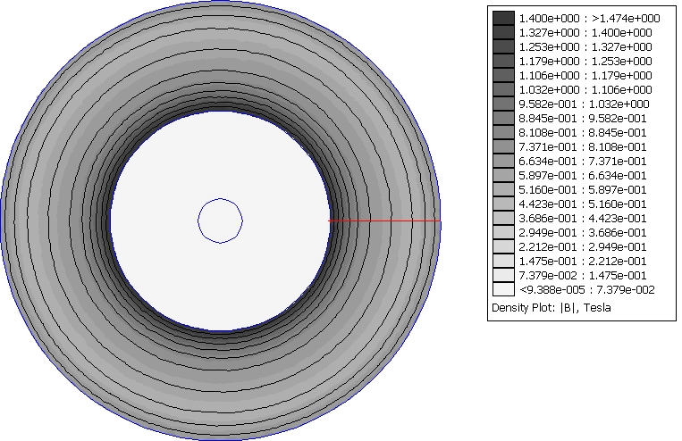
Figure 3: Finite Element Solution.

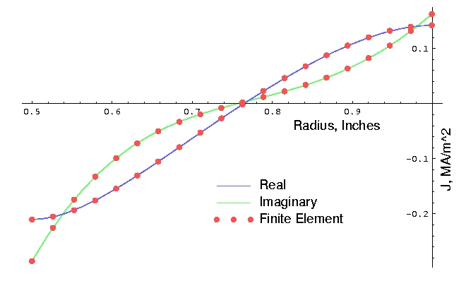
Figure 4: Comparison between finite element and exact results.

A plot of the exact and finite element solutions for current density as a function of pipe radius is shown in Figure 4. RMS error between FEA and exact solution for the test points is 669.5 A/m². To give some idea of what the error means in terms of relative accuracy, the RMS value of the exact solution at the 20 test points considered was 170670. A/m². The RMS error divided by the RMS of the solution is 0.00392, which could be interpreted as a good match.

Conclusions

A benchmark problem with an exact solution was used to test the abilities of FEMM with respect to harmonic problems. Comparing the current density predictions of the finite element model to the exact solution shows a good agreement between the two.

References

R. L. Stoll, The analysis of eddy currents, Oxford University Press, 1974.