Analysis of a Woofer Motor
David Meeker dmeeker@ieee.org
15May2009
1 Introduction
FEMM has been widely used to design speaker motors. Since most speaker motors naturally have an axisymmetric construction, FEMM allows for the computation of the fields and forces in a speaker motor with high accuracy.
This example demonstrates how the program might be used to analyze a typical speaker motor design. For this example, the speaker motor geometry shown in Figure 1 is assumed. The dimensions and materials are roughly the same as those from a 200W 6“ woofer.
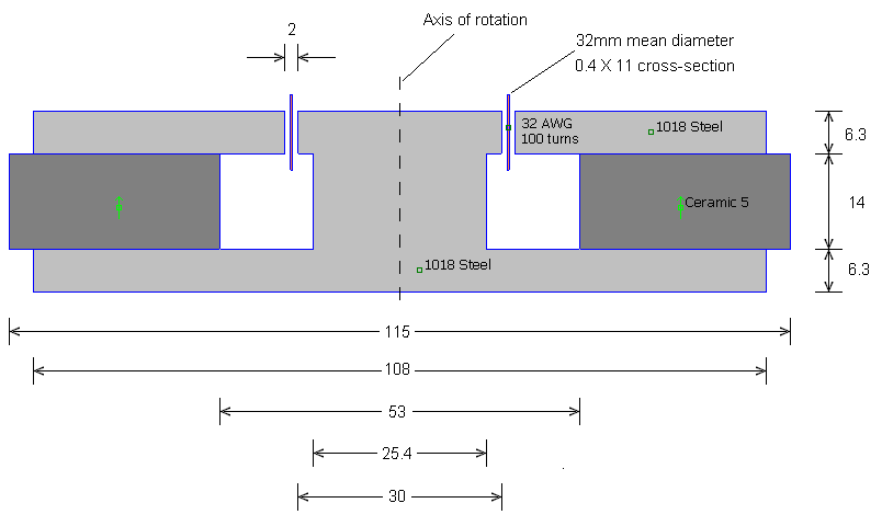
Figure 1: Dimensions of woofer motor cross-section.
2 Woofer Model
A step-by-step model of creating the woofer will not be presented here. The detailed mechanics of constructing the model are nearly identical to the axisymmetric coil presented in the step-by-step Magnetics Tutorial. However, there are a couple of differences in modeling a solenoid and modeling a speaker that will be covered here.
2.1 Permanent Magnet Material
The first difference with the tutorial is that the speaker motor contains a permanent magnet. The permanent magnet material can be added to the model in the same way as “Air” and “18 AWG” materials, i.e. by drag-and-drop from the materials library. In this case, the material to be added is “Ceramic 5”. This material resides in the “PM Materials | Ceramic Magnets ” folder of the materials library. In the model, the material is assigned to a particular block label in the usual way (as described in the tutorial). However, care is needed to define the proper direction of magnetization in the permanent magnet.
The magnetization direction of the permanent magnet can be defined by selecting the block label associated with the permanent magnet material with a left mouse button click when the preprocessor is in Block Label mode ( ). Then, press the space bar to open the selected block label. The “Properties for selected block” dialog will appear. If the material is a permanent magnet material, the “Magnetization Direction” edit box will be active. Enter in a number here to specify the angle of the permanent magnet's orientation, i.e. an angle of 0 directs the magnetization radially outward; an angle of 90 directs the magnetization parallel to the axis of rotation, and so on. Hit “OK” when the proper direction has been entered. The arrow through the selected block label should then select the indicated direction of magnetization. The direction of the arrow always points towards the north pole of the magnet.
2.2 Combine the Voice Coil into a Group
To facilitate moving the voice coil to assess performance at different coil positions, it is useful to assign all the parts that make up the coil to be members of the same group. Then, the group can be selected with one click and moved with a single command.
To put all parts of the voice coil into a group, the preprocessor must first be put into Group mode by pushing the  button. Then push the
  and select all elements in the voice coil (i.e. the segments defining the boundaries of the coil and the block label defining the coil material and turns count). The, press the space bar. The “Group Properties” dialog will then pop up, prompting for a group number to be assigned to the selected items. The default group number is zero, so it would be a good idea to define the group number of items in the voice coil to be 1. In Group Mode, all items in the coil can then be selected by a left mouse button click anywhere near the voice coil.
2.3 Boundary Conditions
The boundary conditions on the edges of the analysis region must be defined so that the boundary definition does not have a spurious effect on the analysis results. For the analysis of speaker motors, the “asymptotic boundary condition” described in the Magnetics Tutorial is sufficient. However, an alternative way of defining an “open” boundary condition is via the “Kelvin Transformation.” The Kelvin Transformation uses a second region linked to the geometry of interest with periodic boundary conditions. If the shape of the second region is selected correctly it can be shown that this region is a mapping of the unbounded region outside the domain of interest into a bounded region that can be analyzed with the finite element method. The advantage of using this technique is that the outer boundary can be placed essentially arbitrarily close to the voice coil without losing accuracy of the solution. With other approaches, the boundary must be a bit farther away.
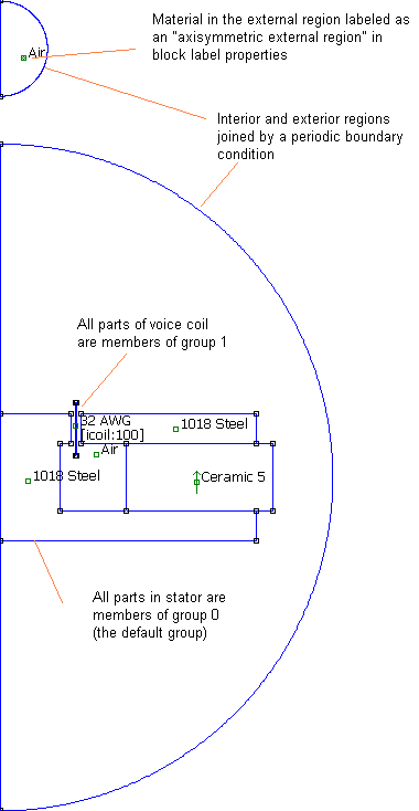
Figure 2: Woofer motor geometry as drawn in the FEMM magnetics preprocessor.
The problem geometry with the Kelvin Transformation boundary condition defined is shown in Figure 2. To build this boundary condition, follow the following steps.
- Draw a half-circle boundary for the “interior” region (i.e. the region where the speaker motor is located).
- Draw a half-circle “exterior” region–meant to represent the rest of the universe aside from the region containing the speaker motor. The exterior region need not be the same size as the interior region.
- Add an extra boundary condition. The type of the boundary condition should be selected as “Periodic”
- Apply the Periodic boundary condition to both the outer edge of the interior and exterior regions.
- Open up the block label placed in the exterior region and make sure the “block label located in an exterior region” is checked. (This check box should be unchecked in all other block labels in the geometry.
- Click on the “Properties | Exterior Region” selection from the main menu. The “Exterior Region Properties” dialog will pop up. Enter the location of the center of the exterior region along the z-axis and the radii of the interior and exterior regions in this dialog.
Anyhow, if the Kelvin Transformation seems too difficult, satisfactory accuracy can also be obtained if a large rectangular region is defined with no boundary conditions explicitly defined on the outer edges, as shown in Figure 3.
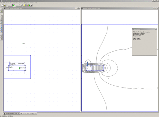
Figure 3: Woofer motor geometry and solution using a distant, square boundary.
3 Analysis Results
To analyze the problem, push the “turn the crank”  button on the preprocessor toolbar. When the analysis finishes, press the “load solution” tool bar button
  to view the results. The resulting solution will look something like that pictured in Figure 4.
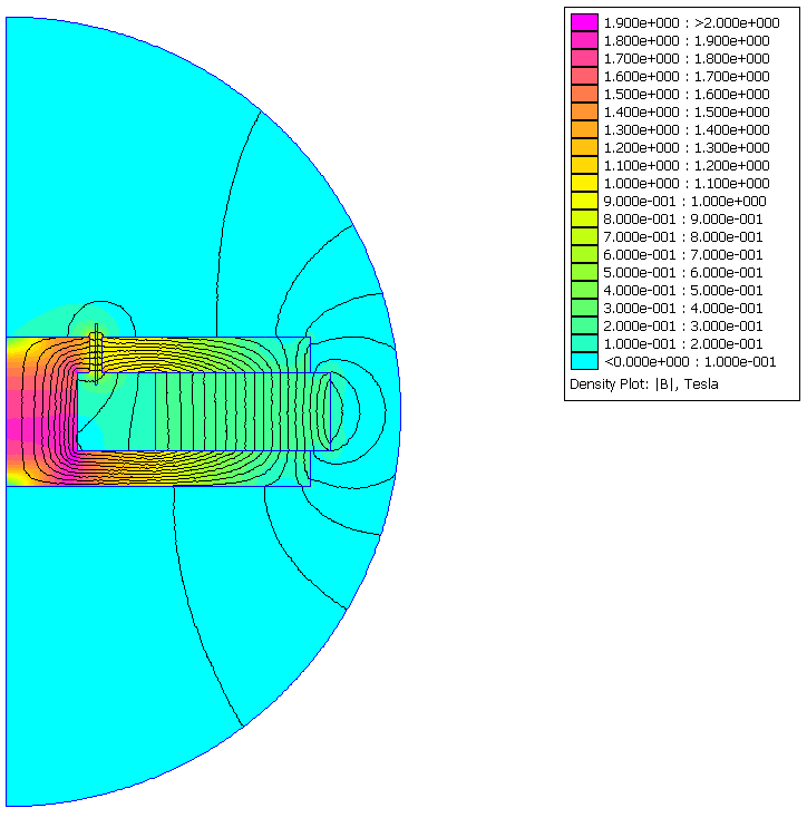
Figure 4: Magnetic field solution as displayed in the FEMM magnetics postprocessor.
However, a picture of the field solution isn't really the objective of the analysis. One typically desires specific performance metrics of the motor.
3.1 Computation of BL
The parameter BL is the gain between an applied current in the coil and a resulting force on the coil. The name “BL” refers directly to the formula for Lorentz force on a wire:
 button. Move the mouse pointer inside the coil region and do a left-button click to select the coil region. The region should light up in green. Then, perform a block integral by clicking the
  toolbar button. A dialog will pop up allowing you to select the type of integral to be performed. Select "Lorentz force (JxB)" from the list and hit "OK". Another dialog will then pop up with the integral analysis result. For this particular example, with the coil in the centered position, the program will report:
r-component: 0 N
z-component: 6.75502 N
For axisymmetric problems, the radial force is always zero (because the solution is, well, axisymmetric). Since a 1A current was applied, the z-component of the force can be directly interpreted as BL, i.e. BL = 6.75502 N/A for this geometry with the coil at its centered position.
3.2 Computation of DC Inductance
For the coil in the Magnetics Tutorial, one can infer the inductance simply by press the Circuit Properties button in the postprocessor
toolbar button. A dialog will pop up allowing you to select the type of integral to be performed. Select "Lorentz force (JxB)" from the list and hit "OK". Another dialog will then pop up with the integral analysis result. For this particular example, with the coil in the centered position, the program will report:
r-component: 0 N
z-component: 6.75502 N
For axisymmetric problems, the radial force is always zero (because the solution is, well, axisymmetric). Since a 1A current was applied, the z-component of the force can be directly interpreted as BL, i.e. BL = 6.75502 N/A for this geometry with the coil at its centered position.
3.2 Computation of DC Inductance
For the coil in the Magnetics Tutorial, one can infer the inductance simply by press the Circuit Properties button in the postprocessor  . For the solenoid in the Tutorial, the "flux/current" result can be directly interpreted as the coil's inductance. For a speaker motor, however, the situation is a bit more subtle. In this case, most of the flux linking the coil comes from the magnet, rather than being due to current in the coil. The magnet flux should be discounted in a computation of self-inductance. A second issue is saturation in the stator flux path. The iron in most speaker designs is usually close to saturation. The reaction field from current in the voice coil is small relative to the field of the permanent magnet. For the purposes of determining the dynamics of the reaction field, the incremental self-inductance about the zero current operating point set by the magnet is what is really of interest.
The incremental self-inductance of the coil can be determined by performing two simulations: a first simulation with 1A of current in the coil, and a second simulation with no current in the coil. In each case, the flux linkage of the coil can be read off of the "circuit property" results. The incremental inductance is simply the difference of the flux linkages in these two cases. For the example geometry, the coil's flux linkage at the centered position with a 1A coil current is -0.0461614 Webers and the flux linkage with a current of 0A is -0.0474315 Webers. The implied self-inductance is:
L = (-0.0461614 Webers - (-0.0474315 Webers))/(1A) = 1.2701 mH
3.3 Computation of DC Resistance
Resistance is reported directly as a "circuit properties" result for the simulation with a 1A coil current. The coil's resistance is the "Voltage/Current" result, reported as 5.40812Ω for the present model.
3.4 Plot of Flux through the Voice Coil
It is also usually of interest to have a quantitative plot of the flux density that links the voice coil. Such a plot can be made in Contour mode. Switch to Contour mode by pressing the
. For the solenoid in the Tutorial, the "flux/current" result can be directly interpreted as the coil's inductance. For a speaker motor, however, the situation is a bit more subtle. In this case, most of the flux linking the coil comes from the magnet, rather than being due to current in the coil. The magnet flux should be discounted in a computation of self-inductance. A second issue is saturation in the stator flux path. The iron in most speaker designs is usually close to saturation. The reaction field from current in the voice coil is small relative to the field of the permanent magnet. For the purposes of determining the dynamics of the reaction field, the incremental self-inductance about the zero current operating point set by the magnet is what is really of interest.
The incremental self-inductance of the coil can be determined by performing two simulations: a first simulation with 1A of current in the coil, and a second simulation with no current in the coil. In each case, the flux linkage of the coil can be read off of the "circuit property" results. The incremental inductance is simply the difference of the flux linkages in these two cases. For the example geometry, the coil's flux linkage at the centered position with a 1A coil current is -0.0461614 Webers and the flux linkage with a current of 0A is -0.0474315 Webers. The implied self-inductance is:
L = (-0.0461614 Webers - (-0.0474315 Webers))/(1A) = 1.2701 mH
3.3 Computation of DC Resistance
Resistance is reported directly as a "circuit properties" result for the simulation with a 1A coil current. The coil's resistance is the "Voltage/Current" result, reported as 5.40812Ω for the present model.
3.4 Plot of Flux through the Voice Coil
It is also usually of interest to have a quantitative plot of the flux density that links the voice coil. Such a plot can be made in Contour mode. Switch to Contour mode by pressing the  button. In this case, the center of the voice coil is located at r=16, z=17.15. Since the coil is 11mm long in the axial direction, it might be insightful to plot the radial flux density on a line from (r=16,z=7.15) to (r=16,27.15). It's possible to place contour points at the nearest node point with a left mouse button click or at the current mouse pointer location with a right mouse button click. However, it's difficult to position the mouse pointer at arbitrary locations with precision. In this case, manual entry of the contour end points can be used. If the
  button to make a plot.
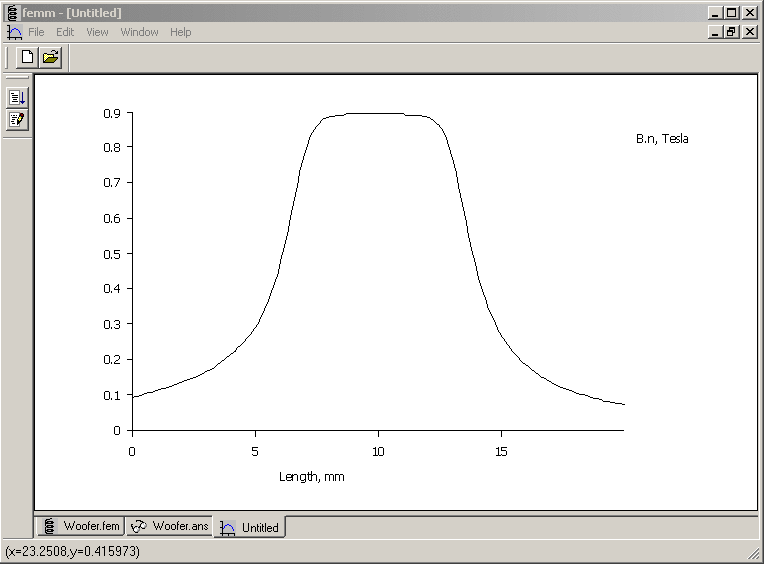
Figure 5: Plot of radial flux density through the voice coil.
The resulting plot is shown as Figure 5. Note the numbers displayed on the left side of the status bar. These numbers indicate the location of the mouse pointer in plot coordinates. Using this tool, it is possible to get approximate field values directly from the plot window, if desired.
4 Automation of Analysis
Section 3 shows how to compute the sort of analytical result that is usually of interest to a speaker motor designer. However, the designer typically desires these quantities to be evaluated at a range of points across the stroke of the voice coil. It would be an onerous chore to repeat the same calculation at many coil positions over several design iterations. However, it is not necessary to manually evaluate the results at each coil position. FEMM supports several different types of scripting that can be used to automate just this sort of repetitive analysis. The available options for scripting are:
- Lua 4.0. The Lua scripting language is built into FEMM and is the engine for all scripting functions. It is possible to write scripts in the Lua language and run them via the “File | Open Lua Script” entry on the FEMM main menu or by pressing the
 toolbar button. Results can be displayed on the Lua console, which can be made visible by pressing the
  button.
 - Mathematica. The MathFEMM package, included in the standard FEMM distribution, allows the control of an instance of FEMM from within a Mathematica session. All scripting functionality that can be implemented directly in Lua is available as “native” Mathematica commands.
- Matlab/Octave. The OctaveFEMM toolbox allows either Matlab or Octave (an open-source Matlab-compatible analysis program) to control an instance of FEMM. Just as with the Mathematica interface, all of the scripting functionality of Lua is available as “native” Matlab/Octave commands.
A script was written to determine the actuator's “BL” and the coils's self-inductance and resistance using each of the three scripting approaches. Because there are so many possible variations in speaker motor geometry, the scripts the speaker motor geometry is not created within the scripts. Rather, the scripts reads an existing geometry info FEMM and analyze it at a number of different coil locations. It is assumed that the speaker motor has been drawn with all elements in the coil belonging to group number 1, so that the voice coil can be easily selected and moved by the notebook. It is also assumed that the .fem file describing the motor is located in the same directory as the notebook.
Mathematica, Matlab, and Octave all have excellent plotting facilities. In these versions of the script, the BL, inductance, and flux density curves are plotted. Examples of the curves plotted by the Mathematica notebook version of the script are shown below as Figures 6-8:
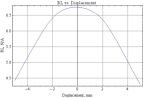
Figure 6: BL versus position
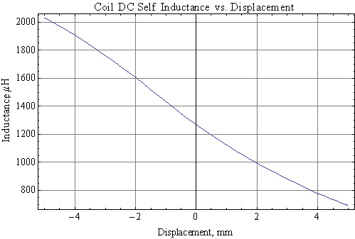
Figure 7: Inductance versus position.
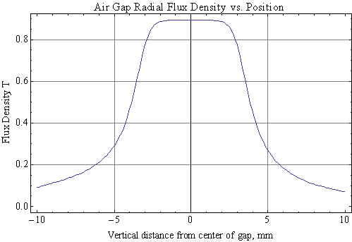
Figure 8: Flux density versus position
5 Files
A number of FEMM models and geometries are associated with this example:
| Woofer.fem | Speaker motor model file |
| Woofer-simple-boundary.fem | Speaker motor model file with simplified boundary condition |
| GetBLCurve.nb | Speaker analysis notebook for Mathematica |
| GetBLCurve.pdf | PDF printout of speaker analysis notebook for Mathematica |
| getblcurve.m | Speaker analysis script for Matlab/Octave |
| getcurve.lua | Speaker analysis script for Lua |
6 Conclusions
An example speaker motor has been used to demonstration the calculation of BL, DC inductance, DC resistance, and flux density in a typical speaker motor. Example scripts for automating the analysis of a speaker motor using the three different scripting methods supported by FEMM have also been presented. In aggregate, these example demonstrate the capabilities of FEMM to compute the DC parameters that are often of interest to speaker motor designers.