Equivalent Thermal Conductivity of Encapsulated Magnet Wire
David Meekerdmeeker@ieee.org
07Oct2021
PDF version
1 Introduction
Many electric machines have a winding consisting of magnet wire potted in an epoxy or silicone encapsulant. The magnet wire typically consists of round copper wire coated with a very thin insulating layer of a material like polyimide or polyamide-imide. The typical problem is shown below in Figure 1.

Figure 1: Encapsulated magnet wire.
To get accurate estimates of operating temperatures, the thermal performance of electric machines is often analyzed by finite element analysis. However, a large number of elements would be needed to directly model the magnet wire and encapsulant, particularly when small gage wire or Litz wire is used. Therefore, an equivalent homogenized thermal conductivity is needed to allow efficient thermal simulations.
Expressions for homogenized thermal conductivity have been presented in previous literature. Many of these works employ the H-S formula for the homogenized representation of bare wires in an encapsulant matrix. The Ollendorff formula [1] (also known as the Hashkin-Shtrikman formula [2]) is accurate for bare wires, but depending on the relative thickness of the insulation, the insulation can have a significant effect on the homogenized conductivity. These previous works have typically dealt with the insulation in several ways:
- Ignore explicit representation of the insulation. The rational is typically that the wires under consideration are big enough that the insulation can be considered negligibly small. [3][4]
- Modify encapsulant thermal conductivity to account for the low thermal conductivity of the insulation [5]
- Employ simple volume fraction / series circuit approach [6]
- Idealize the wire as square to simplify the computation of an equivalent conductivity [7][8]
This note presents the derivation of an equivalent conductivity for an insulated wire that makes no assumptions about the relative thickness of the insulation or the relative conductivities of the wire and insulation. The method is exact for widely separated wires. The equivalent conductivity is then used in combination with the Ollendorff formula to obtain a homogenized thermal conductivity for encapsulated insulated wires. Although the equivalent conductivity for an insulated wire was derived assuming sparsely separated wires, comparisons with 2D finite element analysis (FEA) shows that the resulting homogenized thermal conductivity is accurate over a wide range of copper fill factors for representative insulation and encapsulant materials.
2 Equivalent Conductivity of an Insulated Wire
Consider the geometries shown in Figure 2. On the left of Figure 2 is an insulated wire. The conductor has radius \(R\) and insulation thickness \(\delta\). The thermal conductivities of conductor, insulation, and encapsulant are \(k_c\), \(k_i\), and \(k_p\), respectively. On the right of Figure 2 is a solid wire of radius \(R+\delta\) with an effective thermal conductivity of \(k_w\), which incorporates the effects of the conductor and its insulation. The task is to derive \(k_w\) given the description of the insulated wire.
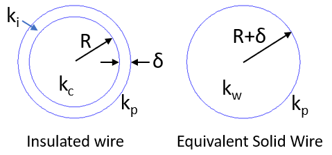
Figure 2: Parameters representing an insulated wire and its equivalent solid-wire representation.
For sparsely spaced wires, a single wire can be considered. Assume that a polar coordinate system indexed by the parameters \(r\) and \(\theta\) has its origin at the center of the wire. Assume that the wire is located in a uniform temperature gradient described by the temperature distribution of \(\ref{uniformgrad}\): \[ \label{uniformgrad} T_\infty = G_\infty \; r \cos{\theta} \] In polar coordinates, the steady-state heat transfer equation to be solved is: \[ \label{lein} \frac{1}{r} \frac{\partial}{\partial r} \left(\,r \frac{\partial T} {\partial r} \right) + \frac{1}{r^2} \left(\frac{\partial^2 T }{\partial \theta^2} \right) + \frac{q}{k} = 0\] where \(k\) is a thermal conductivity and \(q\) is volume heat generation. The associated temperature gradient (\(G\)) and heat flux (\(F\)) are defined as: \[ \label{myGradient} G = - \nabla T\]\[\label{myHeatFlux} F = k G\] Considering only the first harmonic, where the distribution in the \(\theta\) direction is proportional to \(\cos{\theta}\): \[ \label{firstHarmonic} T=\mathcal{T}(r) \cos \theta\] and where there is no heat source (i.e. \(q=0\)), \(\ref{lein}\) simplifies to:
\[ \label{simpoz} \left( \frac{\partial^2 {\cal T}}{\partial r^2} + \frac{1}{r} \frac{\partial {\cal T}}{\partial r} - \frac{1}{r^2} {\cal T}\right) = 0 \] where \({\cal T}\) now just denotes the amplitude of the fundamental.
The solution for \(\ref{simpoz}\) is \[ \label{soln} {\cal T} = \frac{c_1}{r} + c_2 r\] where \(c_1\) and \(c_2\) are to-be-determined coefficients.
2.1 Solid wire of radius R+\(\delta\)
First, consider the temperature distribution in the wire at the right of Figure 2. Following \(\ref{soln}\), the solution for the temperature inside the wire is:\[ \label{inwire1} {\cal T}_1 = \frac{c_{11}}{r} + c_{21} r \] and the solution for the temperature outside the wire is \[ \label{outwire1} {\cal T}_2 = \frac{c_{12}}{r} + c_{22} r \] Inside the wire, the \(c_{11}\) term must be zero, since the temperature cannot be unbounded as \(r \rightarrow 0\). Outside the wire, the \(c_{22}\) term must be equal to gradient \(G_\infty\) to match the constant-gradient solution of \(\ref{uniformgrad}\) far from the wire.
The \(c_{12}\) and \(c_{21}\) terms are yet to be determined. These coefficients can be determined by imposing continuity of temperature and heat flux at the boundary between the wire's outer extent and the encapsulant. Mathematically, these interface conditions can be written as: \[ \label{tcont1} \left. {\cal T}_1 \right|_{r=R+\delta} = \left. {\cal T}_2 \right|_{r=R+\delta}\] \[ \label{dtcont1} \left. k_w \frac{d {\cal T}_1}{dr}\right|_{r=R+\delta} = \left. k_p \frac{d {\cal T}_2}{dr} \right|_{r=R+\delta}\]
Solving these two equations yields: \[\label{4daohc} c_{12} = \frac{G_\infty (k_p-k_w) (R+\delta)^2}{k_p+k_w}\] \[\label{c111} c_{21} = \frac{2 G_\infty k_p}{k_p+k_w}\]
2.2 Wire of radius R with insulation thickness \(\delta\)
Next consider the solution for the temperature in the insulated wire at the left of Figure 2. Instead of two regions, there are now three. Let the solution for the temperature inside the wire be denoted as:\[ \label{inwire2} {\cal T}_0 = c_{20} r \] Inside the insulation, the solution is: \[ \label{inins} {\cal T}_1 = \frac{c_{11}}{r} + c_{21} r \] and the solution for the temperature outside the wire is \[ \label{outwire2} {\cal T}_2 = \frac{c_{12}}{r} + G_\infty r \] Here, we have already taken account that the solution must be bounded at the center of the wire and the solution must go to \(G_\infty r\) at large \(r\).
The \(c_{20}\), \(c_{11}\), \(c_{12}\), and \(c_{21}\) terms are yet to be determined. These coefficients can be determined by imposing continuity of temperature and heat flux at the boundaries between the conductor and the inside of the insulation and between the outside of the insulation and the encapsulant. Mathematically, these interface conditions can be written for the conductor/insulation boundary as:
\[ \label{tcont0} \left. {\cal T}_0 \right|_{r=R} = \left. {\cal T}_2 \right|_{r=R}\] \[ \label{dtcont0} \left. k_c \frac{d {\cal T}_0}{dr}\right|_{r=R} = \left. k_i \frac{d {\cal T}_1}{dr} \right|_{r=R}\]
and for the insulation/encapsulant boundary as:
\[ \label{tcont2} \left. {\cal T}_1 \right|_{r=R+\delta} = \left. {\cal T}_2 \right|_{r=R+\delta}\] \[ \label{dtcont2a} \left. k_i \frac{d {\cal T}_1}{dr}\right|_{r=R+\delta} = \left. k_p \frac{d {\cal T}_2}{dr} \right|_{r=R+\delta}\]
Solving these four equations yields: \[ \label{choad1} c_{20} = \frac{4 G_\infty k_i k_p (R+\delta)^2}{den} \] \[\label{choad2} c_{11} = \frac{2 G_\infty (k_i - k_c) k_p R^2 (R+ \delta)^2}{den} \] \[ \label{choad3} c_{21} = \frac{2 G_\infty (k_i+k_c) k_p (R+\delta)^2}{den} \] \[\label{choad4} c_{12} = \frac{G_\infty (R + \delta)^2 \left( 2 k_i (k_c - k_p) R^2 +\delta (k_c + k_i) (k_i - k_p) (2 R + \delta) \right)}{den} \] where \[ den = 2 k_i (k_c+k_p) R^2 + \delta (k_c + k_i) (k_i +k_p) (2 R + \delta) \]
2.3 Equivalent thermal conductivity for a magnet wire
The equivalent conductivity can be obtained by comparing the temperature at the surface of the wire in the insulated and solid wire cases and solving for the equivalent conductivity that makes the two temperatures equal. Specifically, the \(c_{12}\) coefficients, which represent the surface temperature from \(\ref{4daohc}\) and \(\ref{choad4}\) are set equal to one another and solved for \(k_w\). The resulting \(k_w\), the equivalent homogenized magnet wire thermal conductivity that produces the same temperature as the insulated wire is: \[ \label{mykw} k_w = k_i \left( \frac{2 k_c R^2 + (2 R \delta+\delta^2) (k_c+k_i)}{2 k_i R^2 + (2 R \delta+\delta^2) (k_c+k_i)} \right) \] Note that the encapsulant conductivity, \(k_p\) does not appear in \(\ref{mykw}\) so that the effective conductivity is a property of the insulated wire regardless of the external encapsulant material.
It is interesting to note that if the thermal conductivity of the wire is much greater than that of the insulation and if the insulation is thin compared to the radius of the wire (both typically the case for magnet wire), \(\ref{choad2}\) is well-approximated by \[ \label{approxKw} k_w=k_i \left( \frac{R}{\delta} \right)\]
2.4 Practical ramifications of low insulation thermal conductivity
To get an intuitive feel for the effect of insulation conductivity on the bulk thermal conductivity of the wire, typical wire sizes and thermal conductivities can be considered.
From the ASTM B258 standard [10], the diameter of bare copper wire is defined to be, as a function of American Wire Gauge (AWG) number: \[d(AWG) = 127 \mbox{μm} * 92^{\left( \left( 36-AWG \right)/39\right)}\]. The nominal thickness of magnet wire with single- through quadruple-build can be obtained from manufacturers' literature [11]. Curve fits of the insulation thickness for wire gauges from 14 through 50 are presented in \(\ref{delta1}\)-\(\ref{delta4}\) and graphed versus the nominal values from [11] in Figure 3. \[ \label{delta1} \delta_1 = (28.3357 - 0.250092*AWG - (0.133567*AWG)^2 + (0.0623628*AWG)^3)\mbox{μm} \] \[ \label{delta2} \delta_2 = (65.7318 - 1.72539*AWG + (0.0464358*AWG)^2 + (0.0527203*AWG)^3)\mbox{μm} \] \[ \label{delta3} \delta_3 = (96.5489 - 2.46276*AWG - (0.0629805*AWG)^2 + (0.0695923*AWG)^3)\mbox{μm} \] \[ \label{delta4} \delta_4 = (112.267 - 1.58965*AWG - (0.235476*AWG)^2 + (0.0968019*AWG)^3)\mbox{μm} \]

Figure 2: Manufacturer's nominal magnet wire insulation thickness and best-fit functional approximations.
The thermal conductivities of various magnet wire insulation materials have been tablulated in the literature [12], but the tabulated values span a large range, and the relationship to thermal conductivities measured in practice is not clear. On the basis of this information, 0.26 W/m*K could be taken as a representative value over a wide range of different insulation classes (polyurethane, polyamide/imide, polyamide). The thermal conductivity of copper at room temperature, 398 W/m*K [9], can be taken as a reasonable value. As can be seen in Figure 4, the presence of the insulation drastically reduces the bulk thermal conductivity of the wire versus the thermal conductivity of the wire alone. Furthermore, although heavier insulation may be needed for voltage standoff or mechanical toughness, thermal conductivity is substantially further reduced by these thicker coatings.

Figure 4: Wire conductivity for various wire sizes and insulation thickness
3 Equivalent thermal conductivity for encapsulated magnet wire
Typically, the volume fraction of copper, \(v_c\), is known. However, to use the Ollendorff formula for insulated wire, the volume fraction of insulated wire, \(v_c\), must be computed: \[ \label{myvw} v_w = \left( \frac{(R+\delta)^2}{R^2}\right) v_c \] The Ollendorff formula can then be used to find the effective conductivity of the encapsulated region,\(k_e\): \[ \label{myke} k_e = k_p \left( \frac{k_p (1-v_w) + k_w (1+ v_w) }{k_p (1+v_w) + k_w (1- v_w)} \right) \]
Although the magnet wire's homogenized conductivity, \(k_w\), was obtained assuming widely spaced wires, this representation, when used in the Ollendorff formula, gives an excellent approximation of homogenized thermal conductivity over a wide range of wire fill.
4 FEA comparison to equivalent thermal conductivity
To compare to finite element-derived equivalent thermal conductivity, packing strategy for the wires must be determined. For each packing strategy, an elementary cell must be then be defined. Here, hexagonal packing (i.e. as shown in Fig. 1) and square packing are assumed. The associated elementary cells are shown below in Figure 5. In each elementary cell, the top and bottom are defined to be fixed temperatures \(T_{hi}\) and \(T_{lo}\) respectively. The sides of each cell are thermally insulated by imposing \(dT/dx=0\). In these cells, there is no internal heat generation; heat flows from the top of the cell to the bottom of the cell driven by the fixed-temperature boundary conditions.

Figure 5: FEA domains for hexagonal and square packing comparisons
For each domain the bulk thermal gradient, denoted \(G_b\), is obtained by dividing the temperature drop across the cell by the height of each cell: \[G_b = - \left( \frac{T_{hi}-T_{lo}}{w} \right) \] To obtain the bulk thermal conductivity, the bulk heat flux is needed. To satisfy to Gauss's law (because the sides of the elemental domains are insulated), the average heat flux in the \(y\)-direction must be the same for every value of \(y\). A computationally well-posed way of computing the bulk thermal gradient, \(F_b\), is therefore to take the average of the \(y\)-directed heat flux over the entire domain, which essentially averages the heat flux across every possible choice of \(y\). The resulting bulk thermal conductivity inferred by FEA is then obtained via \(\ref{myHeatFlux}\) as: \[ \label{keFEA} k_{e,FEA} = \frac{F_b}{G_b}\]
For representative geometries, a representative value of encapsulant thermal conductivity must be defined. For a particular application, the choice of an encapsulant involves not just thermal conductivity but also viscosity (so that the part can be potted without air bubbles), operating temperature, mechanical properties of the cured encapsulant, water/chemical resistance, flame resistance, and cost. A selection of encapsulants is listed in Table 1 below, although many other selections are available in the marketplace.
| Material | Type | Therm. Cond. | Viscosity |
|---|---|---|---|
| UR5604 | Urethane | 0.45 W/m*K | 2000 cP |
| EP-6009 | Epoxy | 0.7 W/m*K | 2600 cP |
| SC-305 | Silicone | 0.7 W/m*K | 4000 cP |
| UR-388 | Urethane | 0.7 W/m*K | 6000 cP |
| SC-104 | Silicone | 0.8 W/m*K | 6000 cP |
| BEPU 6608 | Urethane | 0.82 W/m*K | 2000 cP |
| EP-6035 | Epoxy | 1.0 W/m*K | 9500 cP |
| ER2074 | Epoxy | 1.26 W/m*K | 16700 cP |
| EP-340/67 | Epoxy | 1.5 W/m*K | 7000 cP |
| SC-320 LVH | Silicone | 2.1 W/m*K | 4500 cP |
| SC-320 | Silicone | 3.0 W/m*K | 22000 cP |
| SC-320 SLW | Silicone | 3.2 W/m*K | 25000 cP |
As representative properties, 398 W/m*K, 1 W/m*K, and 0.26 W/m*K have been selected for the thermal conductivities of the conductor, encapsulant, and wire insulation, respectively. For single-build insulation with hexagonal packing, the resulting analytical and FEA equivalent thermal conductivities for encapsulated magnet wire are shown in Figure 6 for a wide range of wire sizes and copper fills. Agreemeent is good over all sizes and fills. For the fattest wire (with the thinnest insulation relative to the wire diameter) at the highest fill factor, the error versus FEA is about 3.2%. However, perhaps a better metric is the RMS error over the entire set of comparison points. This RMS error is about 0.35%.

Figure 6: Effective thermal conductivity vs FEA results with hexagonal packing and single-build insulation
Results for square packing are shown below in Figure 7. The agreement with FEA is good at fill below 50%, but error is more pronounced at high fill, with the worst case being about 11% error. The RMS error over the entire dataset is about 1.7%.

Figure 7: Effective thermal conductivity vs FEA results with square packing and single-build insulation
5 Conclusions
A novel analytical expression for the effective conductivity of encapsulated wires has been developed. The expression has good agreement to comparative finite element results when the wires are packed in a hexagon pattern. For square packing, agreement is still good at low fill factors, but larger errors are seen for high fill and large wire sizes (where the insulation thickness is thinner relative to the wire radius).
Error in the square wire case may be driven by the use of the Ollendorff equation. The Ollendorff equation gives bounded results for fill up to 100%, but in the square case, the highest physically obtainable fill for bare wires is \(\pi/4 \approx 78.54\%\). For hexagonal packing, there is less disconnect since the highest physically obtainable fill for bare wires is \(\pi/(2 \sqrt{3})\approx 90.69\%\). Revised versions of the Ollendorff equation for different packing strategies, either analytically derived or regressed from finite element results, would help to improve accuracy at high fill, especially for square packing.
References
[1] F. Ollendorff, “Magnetostatik der Massekerne,” Arch. f. Elektrotechnik., 25, 1931, pp. 436-447. DOI: 10.1007/BF01656937
[2] Z. Hashin and S. Shtrikman, "A variational approach to the theory of the elastic behavior of multi-phase materials," J. Mech. Phys. Solids, 11(2):127-140, 1963. DOI: 10.1016/0022-5096(63)90060-7
[3] H. Cartier and J. Gyselinck, "Homogenization of the winding in thermal finite element modelling of electrical machines," Electric Vehicles International, 03-04 Oct 2019. DOI: 10.1109/EV.2019.8893048 10.1109/EV.2019.8893048
[4] G. S. López et al., "Fast and accurate thermal modeling of magnetic components by FEA-based homogenization," IEEE Trans. Power Electron., 35(2):1830-1844, Feb 2020. DOI: 10.1109/TPEL.2019.2921160
[5] N. Simpson, R. Wrobel, and P. H. Mellor, "Estimation of equivalent thermal parameters of impregnated electrical windings," IEEE Trans. Ind. Appl., 49(6):2505-2515, Nov/Dec 2013. DOI: 10.1109/TIA.2013.2263271
[6] A. A. Woodworth et al., "Creating a multifunctional composite stator slot material system to enable high power density electric machines for electrified aircraft applications," 2018 AIAA/IEEE Electric Aircraft Technologies Symposium, 9-11 Jul 2018. DOI: 10.2514/6.2018-5012
[7] X. Yi et al., "Equivalent thermal conductivity prediction of form-wound windings with Litz wire considering transposition effect," 2019 IEEE International Electric Machines & Drives Conference (IEMDC), 12-15 May 2019. 10.1109/IEMDC.2019.8785368
[8] X. Liu et al., "Effective thermal conductivity calculation and measurement of Litz wire based on the porous metal materials structure," IEEE Trans. Ind. Electron., 67(4):2667-2677, Apr 2020. DOI: 10.1109/TIE.2019.2910031
[9] J. H. Leinhard IV and J. H Leinhard V, A heat transfer textbook, 5th ed., Phlogiston Press, 2020.
[10] "ASTM B258-02 Standard Specification for Standard Nominal Diameters and Cross-Sectional Areas of AWG Sizes of Solid Round Wires Used as Electrical Conductors," ASTM International, 2002. DOI: 10.1520/B0258-02
[11] MWS Tech Book, MWS Wire Industries, May 2016, retrieved 05Oct2021, https://www.mwswire.com/pdf_files/mws_tech_book/techbook2016.pdf
[12] M. Seilmayer and V. K. Katepally, "Thermal conductivity survey of different manufactured insulation systems
of rectangular copper wires," Electronics and Electrical Engineering, 2(1):27-36, July 2018. DOI: 10.3934/ElectrEng.2018.1.27
| File | Last modified | Size |
|---|---|---|
| MagnetWire.nb | 2022-09-05 17:53 | 168Kb |
| MagnetWire.pdf | 2022-09-05 17:52 | 185Kb |
| femmKeHex.nb | 2022-09-05 17:53 | 82Kb |
| femmKeHex.pdf | 2022-09-05 17:53 | 102Kb |
| femmKeSquare.nb | 2022-09-05 17:53 | 69Kb |
| femmKeSquare.pdf | 2022-09-05 17:53 | 102Kb |