Bias Current Linearization Revisited
Abstract: Previously, a generalized bias current linearization was presented for the control of radial magnetic bearings. However, a numerically intensive procedure was required to obtain bias linearization currents. The present work develops an analytical solution to the generalized bias linearization problem in which solutions are indexed by a small number of parameters. The formulation also permits the analytical computation of bias linearization currents for faulted-coil cases.
Keywords: magnetic bearings; actuator force; feedback linearization
1 Introduction
The generalized bias current linearization problem for actuators described by a quadratic current-to-force relationship has been considered by several researchers over the last three decades [1]-[4]. The goal of bias current linearization is to select a set of actuator currents consisting of a bias currents and control currents in each actuator force directions such that that the current required to realize an arbitrary commanded force is a linear combination of those currents, even though the force-to-current relationships are quadratic. Although previous works produced practical solutions to the generalized bias current linearization problem, those solutions were typically the result of computationally intensive numerical algorithms.
The present work presents a closed-form solution to the generalized bias current linearization problem. Manifolds of solutions to the bias current linearization problem are defined via a small number of arbitrarily selected parameters. To derive the solution, the force on a magnetically permeable sphere in free space subject to the magnetic field from an array of coils will be considered. Picking the currents to produce a given force for this case is the same problem is bias current linearization, but the problem naturally has a form that generates a parameterized representation of bias current linearization solutions. Only the solution to a straightforward linear algebra problem is needed to generate the bias current linearization for the permeable sphere problem. Then, radial magnetic bearings with an even number of poles are considered. This problem can be converted to the same convenient form as the permeable sphere, resulting in a manifold of parameterized solutions. Several examples are then considered, showing that the method can produce solutions for magnetic bearings under normal operating conditions and tolerating coil failures.
2 Force on a Magnetically Permeable Sphere
The approach here is somewhat similar to that described in [5]. However, the present case considers a magnetically permeable sphere, whereas [5] considers forces on small permanent magnets. In this case, the sphere's magnetization, \(\mathbf{m}\) is related to the ambient magnetic field intensity, \(\mathbf{H}\) produced by the external coils in the absence of the sphere by [6]:
\[ \label{eq1} \mathbf{m}=\frac{\pi}{2}d^3 \mathbf{H} \] where \(d\) is the diameter of the sphere and it is assumed that the sphere's relative permeability is \(\gg 1\). As in [5], the force, \(\mathbf{f}\), on the dipole is:
\[ \label{eq2} \mathbf{f} = \mathbf{m} \cdot \nabla \mathbf{B} \] Again as in [5], the components of \(\mathbf{m}\) can be represented by a three-component vector, \(m\). The magnetization can then be related to a vector of coil currents, \(i\), by:
\[ \label{eq3} m = M i \] Similarly, the derivatives of flux density, represented in vector form by \(B\), can be represented as the multiplication of the coil current vector by a matrix:
\[ \label{eq4} \begin{eqnarray}
\frac{dB}{dx} & = & D_x i \\
\frac{dB}{dy} & = & D_z i \\
\frac{dB}{dz} & = & D_z i
\end{eqnarray}\] The vector form of force equation \(\ref{eq2}\) can then be summarized as:
\[ \label{eq5} \begin{eqnarray}
i' M' D_x i & = & f_x \\
i' M' D_y i & = & f_y \\
i' M' D_z i & = & f_z
\end{eqnarray} \] Note that the \(M' D_n\) matrix that forms the core of each quadratic force expression is not symmetric. An equivalent symmetric form that would produce the same forces is \( \frac{1}{2} \left( D_n' M + M' D_n \right) \), but the "natural" non-symmetric form lends itself to a very convenient decomposition:
\[ \label{eq6}
\left[ \begin{array}{c} m' D_x \\ m' D_y \\ m' D_z \\ M \end{array} \right] i =
\left\{ \begin{array}{c} f_x \\ f_y \\ f_z \\ m \end{array} \right\}
\] To solve for the currents needed to produce any particular force, vector \(m\) can be selected arbitrarily, essentially parameterizing the solutions. Representing\(\ref{eq6}\) more succinctly as
\[ \label{eq8} G\,i = f \] the solution for the current is:
\[ \label{eq9} i = G^+ f \] where \(G^+\) is the pseudo-inverse of \(G\), since the system is under-determined. There are six rows in \(G\) but typically more than six coil currents to be selected to meet these six constraints. Eq. \( \ref{eq9}\) is a bias linearization solution because the coil currents depend linearly on each desired force component and have a fixed bias component dictated by the choice of \(m\).
The usual ways of generating the current-to-force relationships for radial magnetic bearings (see [1]) result in an indefinite quadratic system of equations typically represented as:
\[ \label{eq10} \begin{eqnarray} i' X_x i & = & f_x \\ i' X_x i & = & f_x \end{eqnarray} \] where \(X_x\) and \(X_y\) are indefinite symmetric matrices. Previously, computation of bias linearization strategies has been approached by solving for bias and force-producing current vectors using numerically intensive procedures. However, if the force matrices could either be derived in or converted to the same form as \(\ref{eq5}\), computation of bias linearization current sets for radial magnetic bearings would be a trivial computation, i.e. \(\ref{eq9}\).
3 Radial Magnetic Bearing with Sinusoidal Flux Variation
Force on the rotor of a magnetic bearing is typically computed using Maxwell's Stress Tensor [7]. Assuming that the rotor's relative magnetic permeability is very high, all flux passes normal to the rotor, and the differential force on the surface of the rotor is:
\[ \label{differentialForce} df = \frac{B^2}{2 \mu_o} \mathbf{n} \] where \(\mu_o\) is the magnetic permeability of free space and \(\mathbf{n}\) is a unit vector pointing outward normal to the rotor. The total force can be obtained
\[ \label{sinFx} f_x = \frac{l\,R}{2 \mu_o}\int_0^{2 \pi} B^2(\theta) \cos \theta d\theta\] \[ \label{sinFy} f_y = \frac{l\,R}{2 \mu_o}\int_0^{2 Pi} B^2(\theta) \sin \theta d\theta\] where \(l\) and \(R\) are the axial length and radius of the rotor, respectively.
Consider the case where the flux density is composed of two sinusoidal components from different harmonics:
\[ B = B_{cj} \cos ( j \theta) + B_{sj} \sin ( j \theta) + B_{ck} \cos (k \theta) +B_{sk} \sin (k \theta)\] where \(j\) and \(k\) are positive-valued integers.
Evaluating \(\ref{sinFx} \) and \(\ref{sinFy}\) yields:
\[ \label{blah} \begin{array}{ccll}
f_x & = & \frac{\pi l R}{4 \mu_o} (B_{cj} B_{ck} + B_{sj} B_{sk} ) & \; \mbox{if} \; |j-k| =1 \\
& = & 0 &\; \mbox{if} \; |j-k| \neq 1
\end{array}\] \[ \label{blahblah} \begin{array}{ccll}
f_y & = & \mbox{sgn}(k-j) \frac{\pi l R}{4 \mu_o} (B_{cj} B_{sk} - B_{sj} B_{ck} ) & \; \mbox{if} \; |j-k| =1 \\
& = & 0 &\; \mbox{if} \; |j-k| \neq 1
\end{array}\] Through the orthogonality of sine and cosine functions, harmonics only interact to produce force if the difference in the order of the harmonics is exactly one. Furthermore, the force solution is a bias linearization solution. The magnitudes of the \(j\) component can be held constant, and the amplitudes of the \(k\) component are linearly proportional to the desired force (or vice versa). For example, if \(k=j+1\), the relationship between flux and force can be written in the same form as \(\ref{eq5}\),
\[ \label{myEqnName1} \left[ \begin{array}{c} m' D_x \\ m' D_y \\ M \end{array} \right] i = \left\{ \begin{array}{c} f_x \\ f_y \\ m \end{array} \right\} \] where
\[\label{myEqnName2} D_x = \frac{\pi l R}{4 \mu_o} \left[ \begin{array}{cccc} 0 & 0 & 1 & 0 \\ 0 & 0 & 0 & 1 \end{array} \right] \] \[ \label{myEqnName3} D_y = \frac{\pi l R}{4 \mu_o} \left[ \begin{array}{cccc} 0 & 0 & 1 & 0 \\ 0 & 0 & 0 & -1 \end{array} \right] \] \[ \label{myEqnName4} M = \left[ \begin{array}{cccc} 1 & 0 & 0 & 0 \\ 0 & 1 & 0 & 0 \end{array} \right] \] \[ \label{myEqnName5} m = \left\{ \begin{array}{c} B_{cj} \\ B_{sj} \end{array} \right\} \] \[ \label{myEqnName6} i = \left\{ \begin{array}{c} B_{cj} \\ B_{sj} \\ B_{ck} \\ B_{sk} \end{array} \right\} \]
More generally, the implication of this result is that the harmonics of flux density can be broken up into even- and odd-numbered harmonics. Even-numbered harmonics can never interact with other even-numbered harmonics, because the difference in order of the harmonics is never equal to one. Similarly, odd-numbered harmonics never interact with other odd-numbered harmonics. The interactions of the harmonics can be cast into the same form as \(\ref{myEqnName1}\) - \(\ref{myEqnName6}\) where the size of the matrices grow to incorporate the extra harmonics considered. If additional harmonics are used, the problem to be solved becomes under-determined and has many solutions in addition to the arbitrary choice of biasing components. Essentially, posing the problem of force on a radial magnetic bearing in terms of interacting harmonics allows the problem to be decomposed into the easy-to-solve form of \(\ref{myEqnName1}\).
4 Current-Controlled Radial Magnetic Bearing
Although the results from the previous section in terms of rotor flux harmonics shed light on how the radial magnetic bearing can be decomposed into an easily bias-linearizable form, magnetic bearings are typically controlled by imposing currents in the bearing coils, not by directly driving flux in the gaps. Furthermore, magnetic bearings are typically idealized as contributions from a number of "point" poles located at even intervals over the surface of the rotor, rather than flux that varies smoothly with position. The objective of this section is to derive an equivalent separation to \(\ref{myEqnName1}\) for this case using the approach of breaking the values of flux density at the bearing's discrete poles into odd and even harmonics.
Consider a non-dimensionalized symmetric magnetic bearing with an even number of poles (similar to the non-dimensionalization described in [9]) where the relationships between dimensional current, gap flux density, and force are related to non-dimensional quantities by:
\[ \label{eq101} i = \left( \frac{\mu_o N}{g B_{sat}} \right ) i_{dim} \] \[ \label{eq102} b = \frac{B_{dim}}{B_{sat}} \] \[ \label{eq103} f = \left( \frac{2 \mu_o}{a B_{sat}^2} \right) f_{dim} \] where \(N\) is the number of turns per pole; \(g\) is the nominal air gap length; and \(B_{sat}\) is the saturation flux density in the bearing iron. A typical magnetic bearing geometry is shown below in Figure 1.
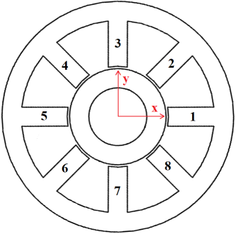
Figure 1: Example 8-pole magnetic bearing layout.
Pole angle \(\Theta\) is defined as:
\[ \label{eq104} \Theta = 360^o \left( \frac{k}{n} \right)_{k=0 \ldots n-1} \]
where \(n\) denotes the number of poles in the bearing. Here, \(n\) is an even number. \[ \label{lambdax} \Lambda_x = \mbox{diag}(\cos(\Theta) ) \] \[ \label{lambday} \Lambda_y = \mbox{diag}(\sin(\Theta)) \] Since there are a set of discrete poles, force can be evaluated via Maxwell's Stress Tensor by summing the contributions from all the poles. This summation is written in matrix form as:
\[ \label{matrixFx} f_x = b' \Lambda_x b\] \[ \label{matrixFy} f_y = b' \Lambda_y b\]
Define matrix \(P\) to be an orthonormal matrix of normalized Discrete Fourier Transform (DFT) basis functions [13] that maps flux density at each of the poles onto the amplitudes of the sine and cosine components at each harmonic:
\[ \label{orthonormal} P=\left[ \begin{array}{c} P_e \\ P_o \end{array} \right] \]
The rows of \(P\) are straightforward to write. The rows of \(P\) either have the form:
\[ \label{eq105} cos(k \Theta)/ \sqrt{cos( k \Theta) cos(k \Theta)'} \] or \[ \label{eq106} \sin(k \Theta) / \sqrt{sin( k \Theta) sin(k \Theta)'} \] depending on whether the row is computing the amplitude of the cosine or sine component of the \(k^{th}\) harmonic. The harmonics are arranged so that the frst set of rows forms \(P_e\), the mappings for even-numbered harmonics and the last rows form \(P_o\), the mapping for odd-numbered harmonics.
Since \( P'P \) is the identity matrix, it can be inserted into \(\ref{matrixFy}\) and \(\ref{matrixFy}\) without affecting the resulting force:
\[ \label{eq107} f_x = b' P' P \Lambda_x P' P b\] \[ f_y = b' P' P \Lambda_y P' P b\] Considering just the inner part of each force relationship and expanding in terms of the even and odd harmonic mappings yields:
\[ \label{eq108} P \Lambda_x P' = \left [ \begin{array}{cc} P_e \Lambda_x P_e' & P_e \Lambda_x P_o' \\ P_o' \Lambda_x P_e' & P_o \Lambda_x P_o' \end{array} \right] \]
Through the orthogonality of discrete sine and cosine series (see Appendix) which behaves in a similar way to orthogonality of continuous sine and cosine functions, \( P_e \Lambda_x P_e' \) and \( P_o \Lambda_x P_o'\) are both zero matrices since only harmonics that are different in order by one can produce a net force:
\[ \label{eq109} P \Lambda_x P' = \left [ \begin{array}{cc} 0 & P_e \Lambda_x P_o' \\ P_o' \Lambda_x P_e' & 0 \end{array} \right] \]
If \(<.,.>\) denotes the inner product, \(<b,Ab>\)=0 for any skew-symmetric matrix \(A\) and vector \(b\).[8] Therefore, an arbitrary skew-symmetric matrix could be added to \(P \Lambda_x P' \) without changing the resulting force. In particular, consider the addition of the particular anti-symmetric matrix:
\[ \label{eq110} P \Lambda_x P' + \left [ \begin{array}{cc} 0 & P_e \Lambda_x P_o' \\ - P_o' \Lambda_x P_e' & 0 \end{array} \right] = \left [ \begin{array}{cc} 0 & 2 P_e \Lambda_x P_o' \\ 0 & 0 \end{array} \right] \] This choice of skew-symmetric matrix performs the simultaneous rank reduction necessary to cast the force relationship into the form of \(\ref{myEqnName1}\).
However, force is ultimately desired in terms of coil currents rather than gap flux. Define matrix \(\cal B\) which converts coil currents to gap flux density as:
\[b={\cal B} i\]
Rolling up the result from \(\ref{eq110}\) into a complete force expression relating current to force yields:
\[ \label{myFx} f_x = i' {\cal B}' \Lambda_x {\cal B} i = i' {\cal B}' P' \left[ \begin{array}{cc} P_e \Lambda_x P_e' & P_e \Lambda_x P_o' \\ P_o \Lambda_x P_e' & P_o \Lambda_x P_o' \end{array} \right] P {\cal B} i = i' P' \left[ \begin{array}{cc} 0 & 2 P_e \Lambda_x P_o' \\ 0 & 0 \end{array} \right] P {\cal B} i = 2 i' {\cal B}' P_e' P_e \Lambda_x P_o' P_o {\cal B} \, i \] and similarly for the y-direction: \[ \label{myFy} f_y = 2 i' {\cal B}' P_e' P_e \Lambda_y P_o' P_o {\cal B} i \]
The force-to-current relationship from \(\ref{myFx}\) and \(\ref{myFy}\) can now be trivially decomposed into the form of \(\ref{myEqnName1}\). The decomposition can be done in two different ways, depending on whether the even- or odd-numbered harmonics are select to form the biasing currents:
\[ \label{paydirt} \begin{array}{ccl}
M & = & P_e {\cal B} \\
D_x & = & 2 P_e \Lambda_x P_o' P_o {\cal B} \\
D_x & = & 2 P_e \Lambda_y P_o' P_o {\cal B} \end{array}
\;\; \mbox{or} \;\;
\begin{array}{ccl} M & = & P_o {\cal B} \\
D_x & = & 2 P_o \Lambda_x P_e' P_e {\cal B} \\
D_x & = & 2 P_o \Lambda_y P_e' P_e {\cal B} \end{array} \] And again, the linear problem to be solved for current to get the desired force is:
\[ \label{myEqnName1redux} \left[ \begin{array}{c} m' D_x \\ m' D_y \\ M \end{array} \right] i = \left\{ \begin{array}{c} f_x \\ f_y \\ m \end{array} \right\} \] where the \(m\) vector of biasing components can be selected arbitrarily. Eq. \(\ref{eq105} \) defines a manifold of possible bias-linearizing solutions depending on the choice of \(m\) and the choice of weighting factors used in building the pseudo-inverse needed to solve the typically under-constrained linear problem.
5 Eight-Pole Radial Magnetic Bearing Example
As a specific example, consider the bias linearization of the 8-pole bearing pictured in Figure 1. For this analysis, it is assumed that the rotor is centered within in the bearing. This bearing has previously been considered in [9]. The relationship between current applied to the coils and flux in the air gaps is determined by matrix \(\cal B\).
\[ {\cal B} = \left[ \begin{array}{cccccccc}
\frac{7}{8} & -\frac{1}{8} & -\frac{1}{8} & -\frac{1}{8} & -\frac{1}{8} & -\frac{1}{8} & -\frac{1}{8} & -\frac{1}{8} \\
-\frac{1}{8} & \frac{7}{8} & -\frac{1}{8} & -\frac{1}{8} & -\frac{1}{8} & -\frac{1}{8} & -\frac{1}{8} & -\frac{1}{8} \\
-\frac{1}{8} & -\frac{1}{8} & \frac{7}{8} & -\frac{1}{8} & -\frac{1}{8} & -\frac{1}{8} & -\frac{1}{8} & -\frac{1}{8} \\
-\frac{1}{8} & -\frac{1}{8} & -\frac{1}{8} & \frac{7}{8} & -\frac{1}{8} & -\frac{1}{8} & -\frac{1}{8} & -\frac{1}{8} \\
-\frac{1}{8} & -\frac{1}{8} & -\frac{1}{8} & -\frac{1}{8} & \frac{7}{8} & -\frac{1}{8} & -\frac{1}{8} & -\frac{1}{8} \\
-\frac{1}{8} & -\frac{1}{8} & -\frac{1}{8} & -\frac{1}{8} & -\frac{1}{8} & \frac{7}{8} & -\frac{1}{8} & -\frac{1}{8} \\
-\frac{1}{8} & -\frac{1}{8} & -\frac{1}{8} & -\frac{1}{8} & -\frac{1}{8} & -\frac{1}{8} & \frac{7}{8} & -\frac{1}{8} \\
-\frac{1}{8} & -\frac{1}{8} & -\frac{1}{8} & -\frac{1}{8} & -\frac{1}{8} & -\frac{1}{8} & -\frac{1}{8} & \frac{7}{8} \end{array}
\right] \] The matrix is close to the identity matrix, but it screens out common mode current due to Gauss's law [10]. Since flux through any closed volume must add up to zero, the only solution for the case in which all poles are trying to push equal flux onto the rotor is for the flux to be zero in all gaps.
As shown in Figure 1, the pole locations are defined as:
\[\Theta = \{0^\circ, 45^\circ, 90^\circ, 135^\circ, 180^\circ, 225^\circ, 270^\circ, 315^\circ \} \]
With these pole locations, the even and odd harmonic mapping matrices can be defined as:
\[P_e = \left[ \begin{array}{c} \frac{1}{2} \cos 2 \Theta \\ \frac{1}{2} \sin 2 \Theta \\ \frac{1}{2 \sqrt{2}} \cos 4 \Theta\end{array} \right] \] \[P_o = \left[ \begin{array}{c} \frac{1}{2} \cos \Theta \\ \frac{1}{2} \sin \Theta \\ \frac{1}{2} \cos 3 \Theta \\ \frac{1}{2} \sin 3 \Theta \end{array} \right] \] Note that \(P_e\) neglects the \(0^{th}\) order harmonic, the common mode that is removed by Gauss's law.
The mapping is then constructed by evaluating \(\ref{paydirt}\), where for this example, even-numbered harmonics are used as the bias space:
\[ \label{exM} M = \left[
\begin{array}{cccccccc}
\frac{1}{2} & 0 & -\frac{1}{2} & 0 & \frac{1}{2} & 0 & -\frac{1}{2} & 0 \\
0 & \frac{1}{2} & 0 & -\frac{1}{2} & 0 & \frac{1}{2} & 0 & -\frac{1}{2} \\
\frac{1}{2 \sqrt{2}} & -\frac{1}{2 \sqrt{2}} & \frac{1}{2 \sqrt{2}} & -\frac{1}{2 \sqrt{2}} & \frac{1}{2 \sqrt{2}} & -\frac{1}{2 \sqrt{2}} & \frac{1}{2 \sqrt{2}} & -\frac{1}{2 \sqrt{2}} \\
\end{array}
\right] \] \[ \label{exDx} D_x = \left[
\begin{array}{cccccccc}
1 & 0 & 0 & 0 & -1 & 0 & 0 & 0 \\
0 & \frac{1}{\sqrt{2}} & 0 & \frac{1}{\sqrt{2}} & 0 & -\frac{1}{\sqrt{2}} & 0 & -\frac{1}{\sqrt{2}} \\
\frac{1}{\sqrt{2}} & -\frac{1}{2} & 0 & \frac{1}{2} & -\frac{1}{\sqrt{2}} & \frac{1}{2} & 0 & -\frac{1}{2} \\
\end{array}
\right]
\] \[ \label{exDy} D_y =
\left[
\begin{array}{cccccccc}
0 & 0 & -1 & 0 & 0 & 0 & 1 & 0 \\
0 & \frac{1}{\sqrt{2}} & 0 & -\frac{1}{\sqrt{2}} & 0 & -\frac{1}{\sqrt{2}} & 0 & \frac{1}{\sqrt{2}} \\
0 & -\frac{1}{2} & \frac{1}{\sqrt{2}} & -\frac{1}{2} & 0 & \frac{1}{2} & -\frac{1}{\sqrt{2}} & \frac{1}{2} \\
\end{array}
\right]
\] The resulting version of \(\ref{myEqnName1redux}\) is under-determined with five linear equations for eight unknowns.
As an example solution, consider the \(m = \{0,0,1\}' \) case. To obtain a power-optimizing solution for the under-determined system, the Moore-Penrose inverse [10] be employed, yielding the power and load capacity optimizing solution presented in [6] and [9]:
\[ \label{optSoln} i= \left(
\begin{array}{c}
0.353553 +0.353553 \, f_x \\
-0.353553-0.25 \, f_x-0.25 \, f_y \\
0.353553 +0.353553 \, f_y \\
-0.353553+0.25 \, f_x-0.25 \, f_y \\
0.353553 -0.353553 \, f_x \\
-0.353553+0.25 \, f_x+0.25 \, f_y \\
0.353553 -0.353553 \, f_y \\
-0.353553-0.25 \, f_x+0.25 \, f_y
\end{array}
\right)
\]
6 Fault Tolerance
Eq. \(\ref{myEqnName1redux}\) can also be used to determine sets of bias linearizing currents that accommodate the failure of one or more coils. Since \(\ref{myEqnName1redux}\) is under-determined, extra equations can be added to the equation to force the current in the failed coils to be zero in the bias linearization solution. Eq. \(\ref{myEqnName1failed}\) is a modified version of \(\ref{myEqnName1redux}\) that incorporates the extra matrix \(A\) defining the failed coil currents:
\[ \label{myEqnName1failed} \left[ \begin{array}{c} m' D_x \\ m' D_y \\ M \\ A\end{array} \right] i = \left\{ \begin{array}{c} f_x \\ f_y \\ m \\ 0\end{array} \right\} \] Continuing the eight-pole example, consider the case in which poles 1, 2, and 4 have failed. In this case, the \(A\) matrix denoting the faulted coils is:
\[ \label{myAmatrix} A= \left[ \begin{array}{cccccccc}
1 & 0 & 0 & 0 & 0 & 0 & 0 & 0 \\
0 & 1 & 0 & 0 & 0 & 0 & 0 & 0 \\
0 & 0 & 0 & 1 & 0 & 0 & 0 & 0
\end{array} \right] \] Although \(\ref{myEqnName1failed}\) has eight equations for eight unknowns in this case, there is still a manifold of possible solutions defined by the arbitrary choice of \(m\).
A reasonable way to select \(m\) is to pick the vector on the basis of minimizing power throughout an entire rotor revolution. Forces are therefore defined as sinusoidal functions of time:
\[ \begin{array}{c} f_x=\cos t \\ f_y=\sin t \end{array} \] A cost function is formed by integrating the squared current through an entire rotation. \[W=\int_0^{2 \pi} i'i dt \] The solution for \(i\) is simple enough that \(W\) can be obtained analytically as a function of \(m\) with Mathematica. Minimization of \(W\) can then proceed using built-in Mathematica minimization routines. A solution that minimizes \(W\) is:
\[m = \{0.6977361206564902, 0.4814466832850557,-0.08407447543994151\}'\]\[
i=\left(
\begin{array}{c} 0 \\
0 \\
-0.762906-0.336945 \, f_x - 0.66034 \, f_y \\
0 \\
0.268076 -0.758061 \, f_x \\
0.170686 -0.758061 \, f_x \\
-0.36449-0.421116 \, f_x+0.66034 \, f_y \\
-0.792207-0.758061 \, f_x
\end{array} \right)
\]
Conclusions
The bias current linearization problem for radial magnetic bearings has been reformulated so that the determination of bias linearization currents can be determined through the solution of a linear problem. This reformulation yields a manifold of analytical solutions indexed by the choice of bias vector magnitude. By imposing additional constraints in the linear algebra problem, faulted currents can be accommodated.
However, it is not clear that the formulation presented in this paper captures all possible bias linearization solution for radial magnetic bearings. The formulation also does not explicitly address unevenly spaced poles or other sorts of (possibly higher-dimensional) bias linearization problems. These solutions could be the focus of future efforts.
References
[1] E. H. Maslen and D. C. Meeker, "Fault-tolerance of magnetic bearings by generalized bias current linearization," IEEE Transactions on Magnetics, 31(3):2304-2314, May 1995.
[2] E. H. Maslen et al., "Fault tolerant magnetic bearings," Journal of Engineering for Gas Turbines and Power, 121(3):504–508, Jul. 1999.
[3] U. Na and A. Palazzolo, "Fault tolerance of magnetic bearings with material path reluctances and fringing factors ," IEEE Transactions on Magnetics, 36(6):3939-3946, Nov. 2000.
[4] U. Na and A. Palazzolo, "Optimized realization of fault-tolerant heteropolar magnetic bearings," Journal of Vibration and Acoustics, 122:209-221, July 2000.
[5] D. C. Meeker, E. H. Maslen, R. R. Ritter, and F. M. Creighton, "Optimal realization of arbitrary forces in a magnetic stereotaxis system," IEEE Transactions on Magnetics, 32(2):320-328, March 1996.
[6] R. Fitzpatrick, "Soft Iron Sphere in Uniform Magnetic Field," Classical Electromagnetism, CreateSpace Independent Publishing, 2015.
[7] H. Woodson and J. Melcher, Electromechanical Dynamics: Fields, Forces, and Motion, Wiley, 1968.
[8] H. Eves Elementary Matrix Theory, Dover Publications, 1980.
[9] D. C. Meeker, Optimal solutions to the inverse problem in quadratic magnetic actuators, doctoral dissertation, University of Virginia, May 1996.
[10] M. Plonus, Applied Electromagnetics, McGraw-Hill, 1978.
[11] J. Barata and M. Hussein, "The Moore-Penrose Pseudoinverse. A Tutorial Review of the Theory", Brazilian Journal of Physics, 42:146-165, Apr. 2012.
[12] J. Smith, Mathematics of the Discrete Fourier Transform (DFT): with Audio Applications, 2nd ed., W3K Publishing, 2007.
[13] S. Smith, The Scientist and Engineer's Guide to Digital Signal Processing, 2nd. ed, California Technical Publishing, 1999.
Appendix: Othogonality of Discrete Sine and Cosine Series
The specific case of interest is the inner product:
\[ \label{forceEq} f = p' \Lambda q \] where \(p\) and \(q\) are vectors associated with the \(m^{th}\) and \(n^{th}\) harmonic of flux around a magnetic bearing rotor and
\[ \label{lbdx} \Lambda = \mbox{diag}(\cos(\Theta) ) \] or \[ \label{lbdy} \Lambda = \mbox{diag}(\sin(\Theta)) \] are diagonal matrices that define the contributions of each pole to the force in a particular force direction where pole angle \(\Theta\) is defined as:
\[ \label{poleAngle} \Theta = 2 \pi \left( \frac{k}{N} \right)_{k=0 \ldots N-1} \] Inner product \(\ref{forceEq}\) can be re-written as an explicit summation with a single index, since \(\Lambda\) is diagonal:
\[ \label{appEq0} f = \sum_{k=0}^{N-1} Z_{k} \] In all, there are six cases to consider, spanning all combinations of cosine or sine distributions for \(\Lambda\), \(p\) and \(q\):
\[ \label{appEq1} Z_{1,k}= \cos \left(\frac{2 \pi k}{N} \right) \cos \left(\frac{2 \pi m k }{N} \right) \cos \left(\frac{2 \pi n k }{N} \right) \] \[ \label{appEq2} Z_{2,k}= \cos \left(\frac{2 \pi k}{N} \right) \cos \left(\frac{2 \pi m k }{N} \right) \sin \left(\frac{2 \pi n k }{N} \right) \] \[ \label{appEq3} Z_{3,k}= \cos \left(\frac{2 \pi k}{N} \right) \sin \left(\frac{2 \pi m k }{N} \right) \sin \left(\frac{2 \pi n k }{N} \right) \] \[ \label{appEq4} Z_{4,k}= \sin \left(\frac{2 \pi k}{N} \right) \cos \left(\frac{2 \pi m k }{N} \right) \cos \left(\frac{2 \pi n k }{N} \right) \] \[ \label{appEq5} Z_{5,k}= \sin \left(\frac{2 \pi k}{N} \right) \cos \left(\frac{2 \pi m k }{N} \right) \sin \left(\frac{2 \pi n k }{N} \right) \] \[ \label{appEq6} Z_{6,k}= \sin \left(\frac{2 \pi k}{N} \right) \sin \left(\frac{2 \pi m k }{N} \right) \sin \left(\frac{2 \pi n k }{N} \right) \]
The goal is to show that, each case, \(\ref{forceEq}\) equals zero when \(|m-n|\neq1\).
Using trigonometric angle sum and difference identities, the six cases can be re-written as:
\[ \label{appEq1a} Z_{1,k}= \frac{1}{2} \cos \left(\frac{2 \pi k}{N}(m-1) \right) \cos \left(\frac{2 \pi n k }{N} \right) + \frac{1}{2} \cos \left(\frac{2 \pi k}{N}(m+1) \right) \cos \left(\frac{2 \pi n k }{N} \right) \] \[ \label{appEq2a} Z_{2,k}= \frac{1}{2} \cos \left(\frac{2 \pi k}{N}(m-1) \right) \sin \left(\frac{2 \pi n k }{N} \right) + \frac{1}{2} \cos \left(\frac{2 \pi k}{N}(m+1) \right) \sin \left(\frac{2 \pi n k }{N} \right) \] \[ \label{appEq3a} Z_{3,k}= \frac{1}{2} \sin \left(\frac{2 \pi k}{N}(m-1) \right) \sin \left(\frac{2 \pi n k }{N} \right) + \frac{1}{2} \sin \left(\frac{2 \pi k}{N}(m+1) \right) \sin \left(\frac{2 \pi n k }{N} \right) \] \[ \label{appEq4a} Z_{4,k}= \frac{1}{2} -\sin \left(\frac{2 \pi k}{N}(m-1) \right) \cos \left(\frac{2 \pi n k }{N} \right) + \frac{1}{2} \sin \left(\frac{2 \pi k}{N}(m+1) \right) \cos \left(\frac{2 \pi n k }{N} \right) \] \[ \label{appEq5a} Z_{5,k}= \frac{1}{2} -\sin \left(\frac{2 \pi k}{N}(m-1) \right) \sin \left(\frac{2 \pi n k }{N} \right) + \frac{1}{2} \sin \left(\frac{2 \pi k}{N}(m+1) \right) \sin \left(\frac{2 \pi n k }{N} \right) \] \[ \label{appEq6a} Z_{6,k}= \frac{1}{2} \cos \left(\frac{2 \pi k}{N}(m-1) \right) \sin \left(\frac{2 \pi n k }{N} \right) - \frac{1}{2} \cos \left(\frac{2 \pi k}{N}(m+1) \right) \sin \left(\frac{2 \pi n k }{N} \right) \]
Orthogonality of Digital Fourier Transform (DFT) sinusoids (see [12]) can then be invoked to understand the conditions for non-zero \(\ref{forceEq}\). Inspecting cases 2, 4, and 6, these cases always yield zero force since cosine and sine series are always orthogonal. For cases 1, 3, and 5, cosines are interacting with cosines and sines are interacting with sines. However, the frequency has to be the same for a non-zero result. Inspecting each of these cases, the frequency can only be the same if \(m-n=1\) (first term in each case yields a non-zero sum and second term yields a zero sum) or if \(n-m=1\) (first term in each case yields a zero sum and second term yields a non-zero sum).
For the case of an even number of poles, eq. \(\ref{forceEq}\) evaluates to the values listed in Table 1 for each of the six cases:
| Case | \(|m-n| \neq 1\) | \(m-n = 1, \, m \neq \frac{N}{2} \) | \(m-n = 1, \, m = \frac{N}{2} \) | \(n-m = 1, \, n \neq \frac{N}{2} \) | \(n-m = 1, \, n = \frac{N}{2} \) |
| 1 | 0 | \(\frac{N}{4}\) | \(\frac{N}{2}\) | \(\frac{N}{4}\) | \(\frac{N}{2}\) |
| 2 | 0 | 0 | 0 | 0 | 0 |
| 3 | 0 | \(\frac{N}{4}\) | 0 | \(\frac{N}{4}\) | 0 |
| 4 | 0 | 0 | 0 | 0 | 0 |
| 5 | 0 | -\(\frac{N}{4}\) | -\(\frac{N}{2}\) | \(\frac{N}{4}\) | 0 |
| 6 | 0 | 0 | 0 | 0 | 0 |
Table 1: Series sum results for each case of sine/cosine combination assuming an even number of magnetic bearing poles.
In every case, \(f=0\) if \(|m-n| \neq 1\). This result allows the set of even-numbered harmonics or the set of odd-numbered harmonics to be selected as bias spaces because \(|m-n| \geq 2\) for each of these sets.
| File | Last modified | Size |
|---|---|---|
| 8PoleSolution.nb | 2019-09-28 18:22 | 54Kb |
| 8PoleSolution.pdf | 2019-09-28 18:22 | 98Kb |
| 8polebrg.png | 2019-09-25 21:55 | 46Kb |
| Actuators25Nov2019.zip | 2019-11-25 06:51 | 3Mb |
| CitedRefs.zip | 2020-02-29 09:06 | 121Mb |
| MoreRefs.zip | 2020-02-29 09:03 | 19Mb |
| NotesOnMoreGeneralFormulation.pdf | 2019-11-13 19:04 | 1Mb |
| OtherRefs.docx | 2020-02-27 22:51 | 19Mb |
| frazier.pdf | 2020-02-29 12:08 | 11Mb |