Bulk "On-Edge" Lamination Material Model
David Meeker
dmeeker@ieee.org
14May2019
Introduction
The purpose of this page is to document the nonlinear DC "on-edge" bulk lamination model used by FEMM. What "on-edge" means is a set of laminations stacked as shown below in Figure 1. Flux flows in the "easy" direction along the laminations and in the "hard" direction across the laminations. For the purposes of this explanation, the vector \(\mathbf{c}_1\) is directed along the easy direction and the vector \(\mathbf{c}_2\) directed along the hard direction. For this note, it is assumed that we are thinking about the laminations in the context of a 2D or axisymmetric magnetic analysis.
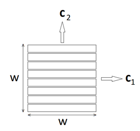
Figure 1: On-edge lamination. (note: c1, c2 now fixed)
One way to model this sort of situation in a finite element solver would be to explicitly model each lamination in the stack. While this method is reasonable for a small number of thick plates with a relatively low fill factor, the number of elements needed to model the geometry could be very large for the case of thin laminations and/or a high fill factor. The goal is therefore to obtain a continuum model of the on-edge lamination stack, essentially representing the laminations as an anisotropic continuum. Then, reasonable results can be realize with a relatively coarse meshing for the continnum region.
Linear Version
For motivational purposes, it is useful to thing about the linear version of the continuum. In this case, there are linear permeabilities in the hard and easy direction that depend on fill factor. As shown in Figure 1, consider an elemental volume with length \(w\) and width \(w\) with a volume iron fill factor represented by \(f\). Equiavalent material properties can then be obtained by considering a parallel magnetic circuit for iron and air reluctances in the "easy" direction and series and and iron and air reluctances. These circuits are shown below in Figure 2.
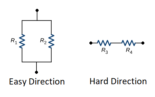
Figure 2: On-edge lamination.
In general, a magnetic reluctance is defined as:
\[R = \frac{length}{\mu * width}\]
where \(mu\) is the magnetic permeability of the reluctance. In this case, the path length and width are both equal to \(w\), simplifying things a bit. In this case, each of the reluctances are defined as:
\[R_1= \frac{1}{\mu \, f}\]
\[R_2= \frac{1}{\mu_o \, (1-f)}\]
\[R_3= \frac{f}{\mu}\]
\[R_4 = \frac{1-f}{\mu_o}\]
where \(\mu_o\) is the permeability of free space.
For the parallel circuit, the combined reluctance is:
\[R_{p}=\frac{1}{1/R_1+1/R_2} = \frac{1}{\mu\, f + \mu_o (1-f)} \]
The reluctance of a \(w \times w\) block of uniform permeability \(\mu_eff\) would be \(R_{eff}=1/\mu_{eff}\). From the definition of the permeability of a uniform region, it can be concluded that the equivalent permeability in the easy direction, \(\mu_1\), is:
\[\mu_1 = \mu\, f + \mu_o (1-f)\]
For the series circuit, the combined reluctance is:
\[R_s = R_3 + R_4 = \frac{\mu(1-f) + \mu_o f}{\mu_o \mu} \]
Using the same equivalent region rationale as above, it can be concluded that:
\[\mu_2 = \frac{\mu_o \mu}{\mu(1-f) + \mu_o f}\]
Some intuitive insight can be gleaned by considering the case where \(\mu \gg \mu_o \). In this case, the equivalent permeabilities simplify to:
\[ \mu_1 \approx f \mu \]
\[ \mu_2 \approx \mu_o/f \]
In the easy direction, the approximate version neglects flux flowing through the parallel air path. In the hard direction, the approximate version assumes that the reluctance in the iron section of the flux path is negligibly small.
Nonlinear Version
For the nonlinear version, it is convenient to neglect the parallel path through air in the easy direction (analogous to the limiting linear case) but to make no simplifying assumption in the hard direction. The easy direction assumption is made to simplify the calculation of the nonlinear operating point. Assume that vector flux density \(\mathbf{B}\) is given. Flux density \(\mathbf{B}\) can be broken into its components along \(\mathbf{c}_1\) and \(\mathbf{c}_2\) as:
\[ \mathbf{B}= B_1 \mathbf{c}_1 + B_2 \mathbf{c}_1 \]
Let \(B_{fe}\) denote the flux density in the isotropic lamination iron. Per the simplifying assumption, since all the flux density in the easy direction flows in the iron, the flux density in the iron easy direction is divided by \(f\). The flux density magnitude in the iron is then:
\[ B_{fe} = \sqrt{ \left( \frac{B_1}{f} \right)^2 + B_2^2} \]
Since the iron is isotropic, the iron part of the field intensity, \(H_{fe}\) is parallel to the iron flux density:
\[H_{fe} = H_n(B_{fe})\left(\frac{B_1}{f B_{fe}} \mathbf{c}_1 + \frac{B_2}{B_{fe}}\mathbf{c}_2 \right) \]
where \(H_n(B_{fe})\) represents the nonlinear B-H curve of the isotropic lamination material. The field intensity across the block is then the sum of the easy direction field intensity directly from \(H_{fe}\) and a weighted sum of field intensities from iron and air in the hard direction, dependent on the fill factor:
\[ H = H_n(B_{fe}) \frac{B_1}{f B_{fe}} \mathbf{c}_1 + \left( f \, H_n(B_{fe}) \frac{B_2}{B_{fe}} + \frac{1-f}{\mu_o}B_2 \right) \mathbf{c}_2 \]
General Anisotropic Material Model
Although the model was derived from a physical model of a lamination, the model could be used to address general anisotropic models. For use in a general anisotropic model, the \(f\) parameter is typically very close to 1. The isotropic B-H curve of the lamination material is then essentiall the same as the response of the bulk anisotropic model with no flux applied across the hard direction.
\[ H_{ez} = H_n\left(\frac{B_{ez}}{f}\right) \approx H_n(B_{ez}) \]
If there is no flux in the easy direction, the field intensity in the hard direction is:
\[ H_{hard} = H_n(B_{hard}) \, f + \frac{1-f}{\mu_o} B_{hard} \approx H_n(B_{hard}) + \frac{1-f}{\mu_o} B_{hard}\]
The \(f\) parameter can then be selected on to produce a least-squares fit to the hard direction B-H curve.
Example Problem
To invoke this material in FEMM, specifiy that the material is "Laminated parallel to x (planar) or r (axisymmetric)" or "Laminated parallel to y (planar) or z (axisymmetric)" in the "Lamination & Wire Type" drop box in the materials definition dialog, as shown below in Figure 3.
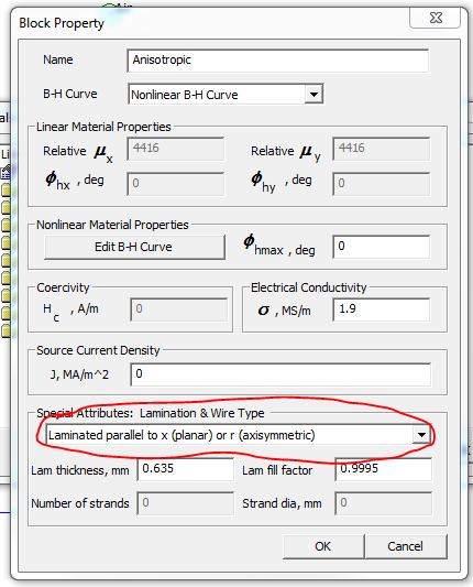
Figure 3: Lamination & Wire Type definition
An example problem, where a fill factor of 0.9995 has been specified in an EI-core inductor is included as induct1a.fem
| File | Last modified | Size |
|---|---|---|
| Capture.PNG | 2019-05-15 06:53 | 33Kb |
| circuits.png | 2019-05-14 19:33 | 18Kb |
| induct1a.fem | 2019-05-15 06:49 | 5Kb |
| small_lam.png | 2019-05-15 10:13 | 7Kb |