
Force on NdFeB disc magnets including eddy current effects
David Meeker dmeeker@ieee.org
February 28, 2007
Introduction
The purpose of this note is to present a low-order dynamic model of the magnetic force on strong rare-earth permanent magnets including time-varying effects. There are generally three effects that impart a history-dependence on magnetic materials [1]:
- Eddy currents.
- Static hysteresis.
- "Excess loss" due to eddy currents which resist domain wall motions at the microscopic level.
Rare earth permanent magnets typically have a permeability that is very nearly the same as air over a wide range of applied fields. This fact implies that the magnetization inside the material is fixed, so that the only relevant loss mechanism in a system solely composed of permanent magnets is eddy currents.
Geometry
The geometry under consideration consists of a relatively thin disc magnet, as shown in Figure 1. The magnet is 1” in diameter and has a 1/8” thickness. The magnet is axially magnetized. The magnet is assumed to be sintered NdFeB-40 magnets with a coercivity of Hc=106 A/m, a remanence of Br = 1.257 T, a density of 0.271 lb/in3, and an electrical conductivity of 0.625 MS/m.
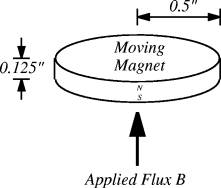
Figure 1: Example geometry.
For ease of notation, the magnet outer radius will be represented by ro and the magnet thickness by h.
It is assumed that the magnet is placed at a fixed location in the field of a coaxial air-cored coil with a prescribed current. The size and location of the coil relative to the magnet are assumed to be uniform enough that a dipole approximation of the magnet is valid.
Eddy current distribution
To create a low-order approximation of the eddy currents, it can be assumed that the distribution of the eddy currents within the magnet is the same as the distribution of currents that is induced in the magnet at low frequencies when the reaction field of the eddy currents can be neglected. Since the magnet is thin, it can also be assumed that the eddy current density is constant across the thickness of the magnet.
If the magnet were exposed to a spatially uniform but time-varying axial field (approximately the form seen by one magnet due to the motion of the other magnet), the low-frequency distribution of eddy currents takes on a relatively simple form. The integral form of Faraday’s law can be applied:
|
|
(1) |
where J represents the current density in the magnet, s represents the electrical conductivity of the magnet, and B represents the applied spatially uniform magnetic field. The implication of Faraday’s law is that the eddy currents flow in a set of concentric loops, as shown in Figure 2.
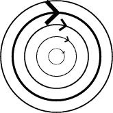
Figure 2: Induced current flow paths in a disc permanent magnet.
For a given radius, r, Faraday’s law can be written as:
|
|
(2) |
which implies the following form for current density when the eddy current’s reaction field is neglected:
|
|
The implication is that a form for the eddy currents in each magnet should be selected that varies linearly with radius.
If the total current across a cross-section of the magnet is defined as i, the form that will hereafter be adopted for J is:
|
|
where i is a current to be determined by the solution of differential equations that will be described later in this note.
Eddy current resistance
To determine the resistance of the eddy current loop, it is first necessary to determine the instantaneous losses dissipated in the magnet due to current i. The losses can be computed by integrating the differential losses over the volume of the magnet:
|
|
(5) |
It can then be noted that the loss is also equal to i2R, where R denotes the eddy current resistance, so that R can be defined as:
|
|
Voltage seen by eddy currents
The definition of current density in terms of total current from (4) can be inserted into (3) to obtain the current induced at low frequencies when reaction field is neglected:
|
|
It can be noted that the induced current should also obey ![]() . By comparing this
relation with (7), the voltage driving the eddy currents can be
obtained:
. By comparing this
relation with (7), the voltage driving the eddy currents can be
obtained:
|
|
It is interesting to note from (8) that the eddy currents are driven by the applied
field as if the eddy currents were a filamentary current loop of radius ![]() .
.
Eddy current self-inductance
It is difficult to obtain an exact value of self-inductance
for the eddy current distribution without the use of a numerical technique like
finite elements. However, a reasonable approximation of the inductance can be
obtained by assuming that the eddy currents are the equivalent of a 1-turn
wound coil with an average radius of ![]() . For a cylindrical
wound coil the "Wheeler Formula" [2]
can be used to closely approximate inductance. Assuming a constant
current density throughout the equivalent coil, to match the resistance of eq. (6), the difference between the inner and outer radii
must also be equal to
. For a cylindrical
wound coil the "Wheeler Formula" [2]
can be used to closely approximate inductance. Assuming a constant
current density throughout the equivalent coil, to match the resistance of eq. (6), the difference between the inner and outer radii
must also be equal to ![]() . In this case, the
Wheeler formula for inductance reduces to:
. In this case, the
Wheeler formula for inductance reduces to:
|
|
To simplify the further mathematics, it can be noted that for the selected aspect ratio (and for all thin disc magnets in general), eq. (9) is closely approximated by:
|
|
(10) |
Force on the magnet with eddy currents
It has been assumed that the ambient field is spatially well-behaved so that a dipole approximation is accurate for calculation of forces. A good representation of a cylindrical hard magnet is as an equivalent cylindrical single-layer coil with Hch amp-turns flowing in the layer of coil. For such a coil, the dipole moment is defined as the coil’s cross-section area times the total amp-turns. If the dipole due to the permanent magnet without eddy currents is denoted as mm, this dipole moment is defined as:
|
|
(11) |
The dipole moment of the eddy current distribution is also
straightforward to compute. Since the
eddy currents appear as a filamentary loop of radius ![]() to the external
field, the dipole moment of the eddy currents (denoted as me)
is:
to the external
field, the dipole moment of the eddy currents (denoted as me)
is:
|
|
(12) |
The total dipole moment of the magnet, m, is:
|
|
Depending on the sign of the induced eddy current i, the apparent magnetization of the magnet can either be bucked or boosted.
The force on the magnet can then be obtained by the standard expression for force on a dipole:
|
|
where z indexes distance along a line through the axis of the magnet.
Time-varying force on the magnet
Now, we have all of the pieces required to solve for force on the magnet, given a specified external magnetic field applied to the magnet as a function of time. The electrical dynamics are described by:
|
|
where L, R, and v are defined in terms of magnet geometry and material properties by (9), (6), and (8), respectively. The force on the magnet is described by (14).
Interesting implications
An interesting result is the time constant related to the eddy current effects. The time constant (denoted as t) is defined as:
|
|
where the more approximate representation has been used to produce a simpler estimation of time constant. This time constant dictates, for example, how long the force takes to settle out in response to a step change in applied field (e.g. it takes a duration of 3t for the force to settle to within 5% of the final value after a step change in applied field). For the particular example magnet under consideration, the time constant per (16) is 5 μs.
Another interesting result is obtained by taking the transfer function representation of (15) and substituting the resulting transfer function to into (13). With some algebraic manipulation, the effective remanence of the magnet (rolling in the effects of eddy currents) can be written as:
|
|
Eq. (17) shows that for a weak applied field, the effects on remanence are negligible. However, for the example magnet, if a large step change in field of 0.32 T is applied, the field of the permanent magnet is momentarily completely cancelled. If the step change in B is instead a step change to –0.32 T, the field of the permanent magnet is instantaneously and momentarily doubled. At even higher field levels, the magnet essentially becomes a "jumping ring"[3], as inductive forces dominate the forces produced via the coercivity of the material.
Conclusions
Eddy current effects in a disc permanent magnet have been considered. By assuming a dipole approximation where appropriate, some relatively simple formulas were derived which indicate the time scale of the eddy current effect, and which can be used to generate a detailed history of force versus time for any applied field. For the example magnet considered, the short time scale of the eddy current effects implies that the eddy current effect is negligible on the time scales and field levels typically considered. However, at high field levels and/or small time scales, the eddy currents will have a discernible effect on force and loss.
References
[1] Jian Guo Zhu, "48531 Electromechanical Systems Lecture Notes," http://services.eng.uts.edu.au/cempe/subjects_JGZ/ems/ems_ch7_nt.pdf
[2] Jim Lux, "Wheeler Formulas for Inductance," http://home.earthlink.net/%7Ejimlux/hv/wheeler.htm
[3] "NCSU Physics Demo Room: Jumping Ring" http://demoroom.physics.ncsu.edu/html/demos/222.html