Permanent Magnet Example
Introduction
The purpose of this example is to demonstrate how the material and direction of permanent magnets are defined in FEMM. For this particular example, a single magnet will be modeled in a 2-D planar geometry
Example Geometry
This example will consider a bar magnet 2 inches long, 1/2 inches wide, and 1/4 inches thick, magnetized through the thickness dimension. The magnet material is N42--the "N" denoting a Neodymium-Iron-Boron (NdFeB) material and the "42" denoting a nominal energy product of 42 MGOe. The magnet is pictured in Figure 1. In the picture, the top side of the magnet is a "N" pole and the bottom side of the magnet (which you can't actually see from this view) is the "S" pole face.

Figure 1: 2" x 1/2" x 1/4" N42 magnet.
Magnet Material Definition
Not every possible magnet material model is pre-defined in FEMM. However, the material model of most permanent magnets can be defined by knowing two quantities:
- The relative magnetic permeability (μr) of the magnet
- The coercivity (Hc) of the magnet
FEMM has a selection of built-in NdFeB materials, but the materials library is not comprehensive. If you want to model a class that is not in the library, you can build you own magnet model in the materials library. A pretty good assumption is that the relative permeability of the magnet is 1.05 (just a touch higher than the magnetic permeability of air). You can then specify the coercivity as:
Hc = 155319 A/m * sqrt(BHmax/MGOe)
So, for example if an N42 magnet were being modeled, the coercivity would be:
Hc = 155319 A/m * sqrt(42) = 1006582 A/m
For example, the material definition for N42 would be as pictured in Figure 2.

Figure 2: Definition of N42 in the FEMM Material Properties Dialog.
Create Geometry
Using the construction methods described in the Magnetics Tutorial, draw the geometry pictured below in Figure 3.

Figure 3: Definition of problem geometry.
This geometry represents a cross-section of the magnet and some air surrounding the magnet. There is a block label inside the magnet and a second in the air around the magnet.
First, open the properties of the block label inside the magnet by selecting it with a left mouse click and pressing <SPACE>. The block property dialog, like shown in Figure 4.

Figure 4: Block Properties dialog.
First, select the previously defined N42 material off of the "Block type" drop list. When a material with a non-zero coercivity is selected (i.e. a material that is a permanent magnet), the "Magnetization Direction" box becomes enabled. It is this box that you use to define the orientation of the magnetism in the permanent magnet. The angle is chosen as depicted in Figure 5. The Magnetization Direction is an angle in units of degrees. The angle is measured from the X-axis. FEMM draws a green arrow representing the magnetization vector, and the arrow points to the North pole of the magnet. In Figure 5, the results of selecting a 90 degree angle are shown. NNN and SSS are superimposed on the drawing to denote the North and South poles of the magnet, respectively. Similarly, if the magnetization angle were selected to be 0, the arrow would point to the right; 180 for an arrow to the left, and 270 for an arrow pointing down.
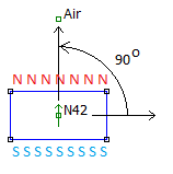
Figure 5: Definition of magnetization angle.
The block label outside the magnet can be set to "Air" with a relative magnetic permeability of 1. In versions 11Oct2012 and later, the program will pick an adequate mesh density for you; otherwise, you should unclick the "Let Triangle choose Mesh Size" box and manually select a reasonable mesh size like, in this case, 0.025".
Boundary Conditions
It's often a good idea to use "Open Boundary Conditions" that make the simulation act as if the analysis were performed on an unbounded domain, rather than a small finite element domain. To do this, click on the concentric circles icon on the toolbar to bring up the "Open Boundary Builder" dialog. Fill out the desired radius of the region (here 1 unit) and the center of the region (here {0,0)). The filled-out dialog is shown in Figure 6. When you click "OK", the program generates a multi-layer "external region" that has the same impedance as unbounded space, even though the domain is finite.
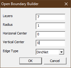
Figure 6: Definition of Asymptotic Boundary Condition.
Solution
For reference, a version of the completed input *.fem file is also available: PMExample.fem
Push the "turn the crank" toolbar button to analyze the solution. When the solver finishes, push the "glasses" toolbar button to view the solution. The solution should look like Figure 7 (at least, when flux density plots are turned on).
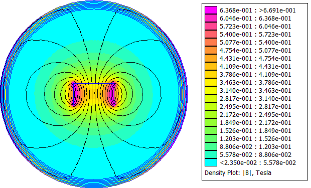
Figure 7: Solution flux lines and field magnitude.
Conclusions
This example showed how to define the magnetization direction of a permanent magnet in FEMM.
It is interesting to note that even though a constant magnetization is applied across the magnet, the resulting field in the permanent magnet doesn't necessarily point along the direction of magnetization. There is a lot of variation in the strength of the field inside the magnet. These additional notes might be interesting with respect to understanding how the operating point of a magnet is related to the magnetization and the energy stored in a permanent magnet:
https://www.femm.info/Archives/misc/BarMagnet.pdf
https://www.femm.info/wiki/PMEnergy
https://www.femm.info/wiki/Analogies