Derivation of Weighted Stress Tensor
David Meeker
27 Aug 2022
Introduction
Maxwell's Stress Tensor [1] is a widely used method of calculating rigid body force and torque in magnetic finite element problems. To evaluate force, one first defines a contour along which the force is computed. The contour should enclose the object of interest. For example, a contour enclosing the rotor of a magnetic bearing is shown in red in Figure 1.
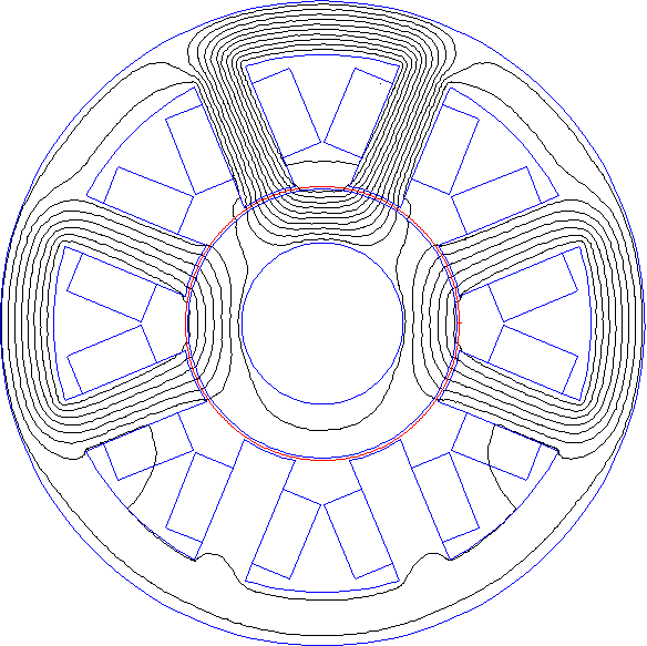
Figure 1: Maxwell Stress integration contour enclosing the rotor of a magnetic bearing.
The Maxwell stress at any point along the contour is \(dF\), a vector quantity:
\[ \label{mst} dF = \frac{1}{2 \mu_o} \left( 2 (B \cdot n) B - (B \cdot B) n\right) \]
where \(B\) is the flux density, \(n\) is a vector perpendicular to the integration contour at the point of interest, and \(\mu_o\) is the magnetic permeability of free space. Similar to the development in [1], for a 2D planar problem, \(\ref{mst}\) can be written explicitly in terms of \(x-\) and \(y-\)directed components as:
\[ \label{dFx} dF_x = \frac{1}{2 \mu_o} \left( \left(B_x^2 - B_y^2 \right) n_x + 2 B_x B_y n_y\right) \] \[\label{dFy} dF_y = \frac{1}{2 \mu_o} \left( \left(B_y^2 - B_x^2 \right) n_y + 2 B_x B_y n_x\right) \]
and the total force is obtained by integrating along the entire length of the contour
\[ \label{Fx} F_x = h \oint dF_x dl \] \[ \label{Fy} F_y = h \oint dF_y dl \]
where \(h\) represents the length of the problem in the into-the-page direction and \(dl\) is a differential length of the contour.
In theory, \(\ref{Fx}\) and \(\ref{Fy}\) should yield the same solution regardless of which contour is picked--so long as that contour encircles the rotor and passes only through air. In practice, since flux density, \(B\), is approximately determined by solving a finite element problem, different choices of contour can yield substantially different force results, especially for coarse meshes. To mitigate the path dependence of the force results, one could take the average force along a lot of different paths through the air gap to average out the error. This is the purpose of the Weighted Stress Tensor method.
Derivation
Various implementations of the multiple integration path idea have appeared in the literature--see [2]-[4]. Here, the method is called "weighted stress tensor" because a weighting function, \(w\), is used to define the paths through the airgap.
First, an area of the finite element domain is defined for which the rigid body force is desired. For ease of nomenclature, we denote the region on which the force is desired as \(\Omega\) and the boundary of that region as \(\partial \Omega\). Then, \(w\) is defined. The weighting function is not unique--it is any continuous function where \(w=1\) on \(\partial \Omega\) and \(w=0\) on all boundaries of the finite element domain and on the boundary of all regions in the finite element solution where \(\mu \neq \mu_o\). The level contours of \(w\) can then be thought of as defining stress tensor integration paths.
To evaluate the force over these multiple integration paths, a direction normal to the contour needs to be defined. A vector that points in the normal direction to any particular path is \(-\nabla w\). We can then substitute the elements of \(-\nabla w\) for the elements of the normal vector in \(\ref{dFx}\) and \(\ref{dFy}):
\[ \label{dfx} df_x = -\frac{1}{2 \mu_o} \left( \left(B_x^2 - B_y^2 \right) w_x + 2 B_x B_y w_y\right) \] \[\label{dfy} df_y = -\frac{1}{2 \mu_o} \left( \left(B_y^2 - B_x^2 \right) w_y + 2 B_x B_y w_x\right) \]
where \(w_x = \partial w / \partial x\) and \(w_y = \partial w / \partial y\). \(-\nabla w\). By integrating \(df\) along a gradient path from the \(\partial \Omega\) to the outer \(w=0\) boundary, we take the average of the force from the continuum of integration paths defined by \(w\). The total force can then be obtained by integrating over the entire region where \(w\) is defined, turning the Maxwell stress tensor line integral into a volume integral:
\[ \label{Fxx} F_x = h \int \int df_x dx dy\] \[ \label{Fyy} F_y = h \int \int df_y dx dy \]
Choice of Weighting function
For stress tensor integration regions with a simple shape like those considered in [2] and [3] (i.e. an annulus or a region between two rectangles), it is straightforward to deduce an analytical form for \(w\). However, for general domain shapes, it is harder to define a weighting function by inspection.
The boundary constraints on \(w\) suggest that a reasonable way to pick \(w\) would be to solve the Laplace equation: \[ \label{Laplace} \nabla^2 w = 0\] subject to the Dirichlet boundary conditions \(w=1\) on \(\partial \Omega\) and \(w=0\) on other material and outer boundaries. This is the calculation that FEMM performs to compute \(w\). The same finite element mesh used to compute the magnetic solution is used to compute \(w\). Since FEMM uses first-order triangles, both the flux density and the gradient of the weighting function are piece-wise constant over each element. For FEMM, the integrations in \(\ref{Fxx}\) and \(\ref{Fyy}\) reduce to simple summations over the elements in the mesh: \[ \label{Fxxx} F_x = h \sum_{k=1}^n df_{x,k} \, a_k \] \[\label{Fyyy} F_y = h \sum_{k=1}^n df_{y,k} \, a_k \] where \(df_{x,k}\) and \(df_{x,k}\) are the force contributions for the \(k^{th}\) element and \(a_k\) is the area of the \(k^{th}\) element.
For the weighting function defined by \(\ref{Laplace}\), a set of level contours of the resuling \(w\) is shown in Figure 2. A close-up of the contours around a single pole is shown in Figure 3. With this definition of \(w\), contributions from every element in the air gap end up folded into the computed force.
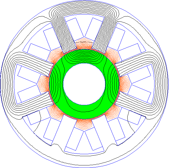
Figure 2: Weighting function showing distribution of Maxwell Stress integration contours.
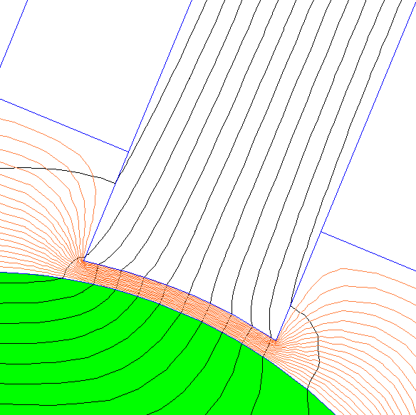
Figure 3: Zoom of Maxwell Stress integration contours with weighting function.
Alternative Weighting Functions
Although the stress tensor contours in Figure 3 look intuitively satisfying, a more detailed examination shows that this definition of \(w\) does not yield the most accurate result. The reason is that elements with high error in \(B\) near corners of the poles (where the solution is nearly singular) end up heavily weighted in the integral, lowering the accuracy of the resulting force calculation.
A simple alternative is to take the Laplace solution for \(w\) and round the computed \(w\) for every node point to either 0 or 1. This strategy selects a single row of elements that runs approximately through the center of the gap as the only contributors to the force result. Since areas with high error are avoided, the accuracy of the resulting calculation is high. For the example problem, the resulting contours are shown in Figure 4. This scheme is the default strategy for generating \(w\) used by FEMM.
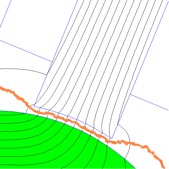
Figure 4: Zoom of Maxwell Stress integration contours with alternate weighting function.
Other alternatives methods for building \(w\) also de-emphasize the contributions of high error regions. Instead of solving a \(\ref{Laplace}\), one can define a fictitious material property, \(\rho\), and solve the differential equation: \[\nabla \cdot (\rho \nabla w) = 0\]. Property \(rho\) could be based on element size or on some a posteriori estimate of error in the finite element mesh so that \(w\) avoids regions of high error in the original finite element solution.
FEMM has five different options for \(\rho\) that can be selected via the Preferences | Magnetics Output dialog. The choices are:
Option 1: \(\rho = 1\). This is the original Laplace equation solution.
Option 2: \(\rho_k = \sqrt{a_k}\). This approach prefers elements with large areas. Since the mesh is refined around corners and areas with high error, this scheme tends to avoid regions of high error.
Options 3 and 4: \( \rho \) selected based on different error metrics.
Conclusions
This note has explained FEMM's Weighted Stress Tensor approach. By effectively taking the average over many stress tensor paths, error is lower than a line integral computed along a single path. No field smoothing is needed to implement the method.
Although this treatment just considered the case of 2D planar magnetostatic problems, the method readily generalizes to axisymmetric and/or AC problems.
References
[1] Y. S. Kim, "Electromagnetic Force Calculation Method in Finite Element Analysis for Programmers", Universal Journal of Electrical and Electronic Engineering, 6(2B):62-67, May 2019
[2] S. McFee, J. P. Webb, and D. A. Lowther, “A tunable volume integration formulation for force calculation in finite-element based computational magnetostatics,” IEEE Transactions on Magnetics, 24(1):439-442, January 1988.
[3] F. Henrotte, M. Felden, M. vander Giet and K. Hameyer, "Electromagnetic force computation with the Eggshell method," Proceedings of the 14th International IGTE Symposium on Numerical Field Calculation in Electrical Engineering, 19-22 Sep 2010.
[4] A. Arkkio, Analysis of Induction Motors Based on the Numerical Solution of the Magnetic Field and Circuit Equations, Doctoral Dissertation, Helsinki University of Technology, 1987.
| File | Last modified | Size |
|---|---|---|
| IntegrationPath.png | 2022-08-27 15:12 | 36Kb |
| RadialMagneticBearing.fem | 2022-08-28 13:30 | 10Kb |
| WeightingFunction.png | 2022-08-27 15:12 | 42Kb |
| WeightingFunctionZoom.png | 2022-08-27 15:12 | 25Kb |
| WeightingFunctionZoomAlt.png | 2022-08-28 12:25 | 16Kb |