Rotating Losses in a Surface Mount Permanent Magnet Motor
David Meeker
dmeeker@ieee.org
18Oct2017
1 Introduction
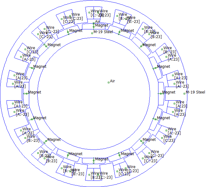
This note considers the analysis of a surface-mount permanent magnet motor with a concentrated winding. Although only a few winding schemes are widely used (1/4 or 2/7 slots per pole per phase), a great variety of concentrated windings are possible, as shown in [1]. The present example uses a 3/8 pitch winding with 16 magnets and 18 stator slots, shown in Figure 1. Although the stator teeth are straight, the motor has very low cogging torque (~1% per unit) and very low harmonic distortion of the back EMF waveform (~1% THD). This motor could be used in precision direct-drive servo applications where precise control over the motor is required. The motor would most likely run in combination with a field oriented controller, driving the motor with currents that are sinusoidal over time.

Figure 1: Motor with 3/8 pitch.
However, the wide slot openings could cause substantial losses in the magnets, especially as speed increases. Flux density in the iron is also relatively high, implying non-negligible core losses. To understand how the motor would work across a wide range of frequencies, a calculation of core, magnet, and winding losses under load and at speed is needed.
This example will show how a series of FEMM solutions (e.g. a simulation at one degree steps around an entire rotation) can be used to compute core losses in this challenging structure. Matlab scripts will be used to control the series of batch FEMM runs.
2 Motor Construction
The magnet material is N42UH with a nominal coercivity of Hc = 1,007,000 A/m and a relative permeability of 1.0277. The electrical conductivity of the magnet material is 0.556*106 S/m.
The core material is DI-MAX M-19 non-oriented silicon steel laminations. The laminations are 29 gauge with a thickness of 0.355 mm. In this example, both the stator and the rotor core are constructed of stacked and bonded laminations. However, the rotor core of SPM machines is often machined out of a single piece of low carbon steel. Here, a laminated rotor core is assumed for tutorial purposes, to show how losses are computed on moving rotor laminations.
The rotor ID is 1.425" and the rotor OD is 1.790". The clearance between the magnets and the stator surface is 0.015". The width of each stator tooth is 0.170". The stator OD 2.376". The diameter of the stator tooth root is 2.216". The axial length of the magnets, rotor core, and stator laminations is 0.3".
The wire is heavy build Polyimide-ML insulated AWG 25 magnet wire. There are 23 turns wrapped around each stator tooth in a 3/8 pitch winding pattern. It is estimated that the average end turn length is 0.4" on each side of each coil, such that the stator resistance will be a factor of (0.4" + 0.3")/(0.3") = 2.333 times the resistance computed from a purely 2D simulation.
3 Core Loss Model
There are a number of methods for estimating the core losses of an electric machines. As explained in [2] and [3], a consistent way is to incorporate a model of the core loss mechanisms (eddy currents, hysteresis, and excess loss) into the B-H relationship used in a time-transient model, such the effects of the core losses are directly visible as perturbations to voltage and current at the terminals of the machine. Unfortunately, it can be very difficult to create and time-consuming to run such a model. A commonly used alternative approach (referred to as the "Traditional Technique" in [2]) is to infer an estimate of core losses from the post-processing of a series of essentially magnetostatic runs that ignore the loss mechanisms in the computation of the magnetic field. This approach assumes that because the core is laminated, the core losses will have only a small effect on the field distribution so that reasonably accurate estimates of the field distribution can be obtained by neglecting losses.
In the "Traditional Technique," losses are then inferred from the computed magnetostatic field distribution using experimentally obtained loss data. To aid in the application of this experimental data, it is useful to fit the experimental loss data to a simple, empirical, functional form so that the losses can be quickly evaluated given a particular flux magnitude and frequency. This section will take core loss data from manufacturer's data sheets and converts it into an empirical form that can be directly applied to core loss calculations.
3.1 Core Loss Data
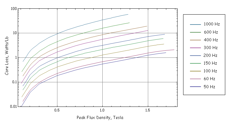
Material property data is required as a basis for core loss calculations. A grade of silicon core iron that is both high quality and commonly available is M-19. Loss data for M-19 is shown below in Figure 2 for a 29-gauge sheet (0.014" thick).

Figure 2: Core loss curves of 29-gauge sheet.
For the purposes of loss computation, it is useful to have a simple form that approximately captures the entire range of curves. A "traditional" way to do this is to assume that the core loss can be broken into a part due to hysteresis, which varies linearly with frequency, and a part due to eddy currents, which varies with the square of frequency:
| Pcore = Ph + Pe = Chω B2 + Ceω2 B2 | (1) |
where Ph and Pe are hysteresis loss and eddy current loss, respectively. Parameters Ch and Ce are hysteresis and eddy current loss coefficients that are regressed from the core loss data. The B in the formula is the amplitude of the flux density (i.e. the peak value).
A reference for the "classical" derivation of core loss separation is [4]. A more modern discussion is contained in [5]. The simple form of (1) is employed here because a curve fit to this form yields reasonable accuracy over the range of application in the problem under consideration.
A reasonable fit to the data for 29-gauge M-19 from 50Hz to 600 Hz is:
| Ch = 0.00844 Watt/(lb*Tesla2*Hz) |
| Ce = 31.2*10-6 Watt/(lb*Tesla2*Hz2) |
For the purposes of finite element calculations, however, we are interested in loss per unit volume, not loss per unit weight. The density of M-19 is:
ρ = 7.70 gm/cm3
If the density is used to convert between loss per unit weight and loss per unit volume, the loss is:
| Ch = 143 Watt/(m3*Tesla2*Hz) |
| Ce = 0.530 Watt/(m3*Tesla2*Hz2) |
3.2 Lamination Stacking Factor
Laminations always have a stacking factor of less than 100%. Various estimates of stacking factor versus lamination thickness are compiled on the StackingFactor page. On the basis of this guidance, 95% is a reasonable assumption for the stacking factor of 0.014" laminations. To account for the effect of the stacking factor, it can be noted that the entire loss (in this estimate) scales by B2. We'd expect that the concentration of flux would increase the loss inside the lamination by (1/StackingFactor)2. However, the iron per unit volume also goes down—there's less iron per unit volume to generate losses, which gives back a factor of StackingFactor. Overall, the stacking factor can be incorporated in the loss by simply dividing the loss formula by the stacking factor of 0.95:
| Pstack = (151 ω Bm2 + 0.558 ω2 Bm2 ) W/m3 | (5) |
Eq. (5) is the equation to use for loss per volume in the machine under consideration.
3.3 Multiple Harmonics
The flux versus time predicted by the finite element model will not be sinusoidal, because it will be including all effects of the motor's geometry as the rotor moves past the stator. If the stator steel were described by linear material properties, the losses could be rigorously decomposed into elements occurring at different frequencies which are summed to obtain the total loss. Even though the material properties are not linear, a widely used approximate method of estimating core losses is to assume that the losses can still be decomposed into multiple components occurring at multiple time harmonics. The core loss expression can then be applied to the each harmonic and the results summed to obtain an approximation of the total core loss. Mathematically, this approach can be represented as:
| (6) |
where Bm is the amplitude of the mth time harmonic of the base frequency, ω.
4 Proximity Loss Model
For some machines, proximity effect losses can significantly increase the copper losses. In AC problems, as shown in [6], a region with wires can be replaced by a homogenized region with a complex-valued permeability. The imaginary part of the permeability is associated with the losses. Though [6] presents a fitting function that computes losses across a very wide range of frequencies and fill factors, the situation most likely to be encountered in typical motor applications is the low frequency limiting case. In the low frequency case, the loss has a much simpler form. The proximity loss per unit volume, Pprox, is:
| Pprox = Cproxω2 B2 | (7) |
where Cprox is a loss coefficient that can be gleaned from the Appendix of [6]:
| Cprox = fill (π2/8) σwire dwire2 | (8) |
where σwire and dwire are the electrical conductivity and diameter of the conductor wires, respectively. Note that the form of (7) is very similar to the eddy current losses in laminations. Using this model, losses in wound regions can be totaled up over frequency and space in exactly the same fashion as core losses in the laminations, simply using different values for the core loss coefficients (i.e. Ce = Cprox, Ch = 0).
5 Magnet Loss Model
Magnet loss is computed like in [7]. In this method, the reaction field of the eddy currents is ignored, and the current density, Jm in the magnet cross-section is:
| Jm = -σm dA/dt + Jc | (9) |
where Jc is a constraint current density selected to make the total current in the cross-section of each magnet equal to zero and σm is the electrical conductivity of the permanent magnet material. The loss is then obtained by integrating Jc2/σm over the volume of each magnet.
Similar to the losses for the core, it is easier in the script to break A into a number of harmonics so that at each harmonic,
| Jm = -σm j ω A + Jc | (10) |
The losses are then computed for each harmonic and summed over all harmonics to get the total loss.
6 Loss Calculation
The methods described in the previous sections can be used to compute core, magnet, and proximity effect losses in the machine under load. However, many finite element runs must be performed to collect the information necessary to apply the loss equations throughout the machine so that the total losses can be computed. The mo_numnodes, mo_numelements, mo_getnode, and mo_getelement commands that were added in the 15Jul2009 release of FEMM provide the element-level access to the mesh that is necessary to keep track of the flux density vs. rotor angle in each element of the laminated iron.
To collect and analyze the requisite flux density vs. time information, a (heavily commented) Matlab script was created (script mySPMLossScript.m that operates on model my_SPM_motor.fem). The script performs a series of finite element runs, incrementing the rotor position and stator currents with each successive run and collecting the required data on the magnetic fields in rotor, stator, magnets, and coils.
To keep track of which loss mechanism applies to each section of the model, different regions of the model are assigned to specific groups. The script assumes the region grouping listed in Table 1.
| Region | Group |
| Air | 0 |
| Stator Core | 1 |
| Windings | 2 |
| Rotor Core | 10 |
| Magnets | 11...26 |
Table 1: Grouping of model regions for loss calculation.
During the first run of the series, the script performs some additional bookkeeping that is needed to locate the points at which the magnetic field is to be evaluated during subsequent iterations of the script. The location of the centroid and the size of each element contained in a laminated region is recorded for later use. As the rotor's position is changed, the finite element mesh changes. The element centroids from the initial finite element mesh are fixed points in the lamination geometry at which the field is evaluated in each incremental analysis, regardless of remeshing.
The flux density is then evaluated at every stored element centroid for every rotor position, essentially building up a history of flux density versus time for each element in the laminated regions. Some extra care is required for points located in the rotor. The initial centroid locations need to be rotated through the same angle as the rotor so that the rotor field is always evaluated at the same points on the rotor from run to run. The resulting field evaluations also need to be rotated so that the field is for points on the rotor is always represented in the same rotor-fixed reference frame.
Care must also be taken to evaluate the performance over a suitably broad range of angles. In particular, concentrated windings like the one considered in this example can have significant sub-harmonics of significant amplitude, and a big enough angle must be considered to capture the effects of the winding sub-harmonics on rotor losses. For example, the winding factor for various harmonics in the selected 3/8 winding is shown below in Table 2. For this winding, there is significant content on the 2nd harmonic. To properly account for all induced currents in the magnets, the example machine must therefore be evaluated over 180 of rotor motion to expose the rotor magnets to the complete stator winding waveform.
| Harmonic | Winding Factor |
| 1 | 0 |
| 2 | 0.0606617 |
| 3 | 0 |
| 4 | 0.13985 |
| 5 | 0 |
| 6 | 0 |
| 7 | 0 |
| 8 | 0.945214 |
| 9 | 0 |
| 10 | 0.945214 |
| 11 | 0 |
| 12 | 0 |
| 13 | 0 |
| 14 | 0.13985 |
| 15 | 0 |
| 16 | 0.0606617 |
| 17 | 0 |
| 18 | 0 |
| 19 | 0 |
| 20 | 0.0606617 |
| 21 | 0 |
Table 2: Winding Factor vs. Harmonic for a 3/8 winding with 18 slots and 16 magnets.
Once finite element runs have been performed over a suitably large arc, Matlab's built-in Fast Fourier Transform (fft) function is used to turn what is essentially a time series of flux densities at each element centroid into amplitudes of various harmonics of flux density, as required by (6) for the evaluation of losses. The contributions from all harmonics for all elements are then added up to get the total core and proximity effect losses. FFTs of the vector potential in the magnet are also used to compute the loss at each harmonic.
7 Loss Results
Running the core loss script with a phase current amplitude of 2A positioned in-phase entirely aligned with the machine's Iq axis, the script produces the following loss results at the 4000 RPM base speed:
rotor speed = 4000 RPM
mechanical power = 62.2952 W
rotor core loss = 0.0574995 W
stator core loss = 3.40587 W
prox loss = 0.0585815 W
i^2 R loss = 4.37018 W
magnet loss = 1.38116 W
total electromagnetic losses = 9.27329 W
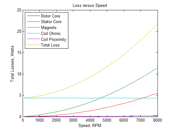
The losses computed by the script over a wide range of speeds is shown below as Figure 3. Only one set of finite element runs is needed to infer the results for all speeds.

Figure 3: Plot of loss components versus speed for a 2A motor current.
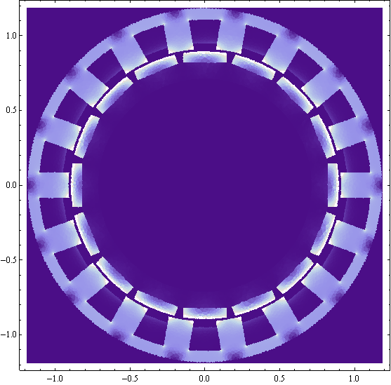
The power loss density can be plotted out into a heating map of the motor, as shown in Figure 4. White color represents high losses; low/no loss is represented by a dark color. This analysis shows that although the magnets are a relatively small portion of the loss, the loss density in the magnets is the highest of anywhere in the motor. In the stator, the highest losses are in the pole tips, though the losses are fairly uniform throughout the stator. A small amount of proximity effect loss is in evidence on the surface of the coils nearest to the air gap.

Figure 4: Plot of loss power density due to eddy currents and hysteresis throughout the motor at 4000RPM.
8 Conclusions
An example has been presented in which FEMM is used compute the core, magnet, winding losses of a permanent magnet motor under load. A more complete analysis could also consider windage and bearing losses. A more complete thermal analysis of the motor would also help to determine the actual operating temperature of the machine, which influences the ohmic losses in the windings and the flux sourced by the permanent magnets. Some additional consideration of end effects might also be warranted, since the example machine has a relatively short axial length. In particular, the proximity effect losses could be higher due to proximity losses in the end turns, and the magnet losses could be a bit lower because of resistance of the "end turn" portion of the current flow paths in the magnets.
Note that the example script runs with the "smart mesh" feature turned on. "Smart mesh" is the default configuration of FEMM, which typically ensures that there is an adequately dense mesh for accurate force and loss calculation. However, the mesh for a full machine tends to have several 10's of thousands of nodes, so the entire loss calculation run takes a few hours to complete. If smart mesh is turned off (change to smartmesh(0); on line 68 of the script), the analysis runs much faster, but the result is less accurate. Loss results tend to be a bit higher because numerical noise associated with the coarse mesh is interpreted as lossy high frequency flux density.
Although there are many different PM machine geometries, the script used to compute the core, magnet, and winding losses for this machine should be readily adaptable for use in other permanent magnet machine geometries (e.g. outrunner surface mount machines, interior permanent magnet machines, and so on). The parameters that need to be changed to consider other machines are generally confined to the User-Defined Parameters portion of the loss script. However, changes might be needed in the portion of the code that maps DQ reference frame currents onto the phase currents, depending on the initial position of the rotor and the layout of the phase windings.
Lastly, the present implementation does not take advantage of parallel processing capabilities that could be used through Matlab. Since the evaluation at each angle has no dependence on other solutions, the script could be re-arranged to use parfor to evaluate multiple rotor positions at the same time using multiple instances of FEMM.
References
[1] F. Libert, J. Soulard, "Investigation on pole-slot combinations for permanent-magnet machines with concentrated windings", KTH Report, 2004.
[2] E. Dlala, "Comparison of models for estimating magnetic core losses in electrical machines using the finite-element method," IEEE Transactions on Magnetics, 45(2):716-725, Feb. 2009.
[3] H. Trabelsi, A. Mansouri, and M. Gmiden, "On the no-load iron losses calculations of a SMPM using VPM and transient finite element analysis," International Journal of Sciences and Techniques of Automatic Control & Computer Engineering, 2(1):470-483, July 2008.
[4] R. L. Stoll, "The analysis of eddy currents," Oxford University Press, 1974.
[5] D. M. Ionel et al. "On the variation with flux and frequency of the core loss coefficients in electrical machines," IEEE Transactions on Industry Applications, 42(3):658-667 May/June 2006. (http://eprints.gla.ac.uk/3438/)
[6] D.C. Meeker, "An improved continuum skin and proximity effect model for hexagonally packed wires," Journal of Computational and Applied Mathematics, 236(18):4635-4644, Dec. 2012. http://dx.doi.org/10.1016/j.cam.2012.04.009
[7] D. Ishak, Z. Q. Zhu, and D. Howe, "Eddy-current loss in the rotor magnets of permanent-magnet brushless machines having a fractional number of slots per pole," IEEE Transactions on Magnetics, 41(9):2462-2469, Sept. 2005.
| File | Last modified | Size |
|---|---|---|
| myLossResults.csv | 2017-10-19 10:56 | 8Kb |
| mySPMLossResults.nb | 2017-10-17 21:47 | 1Mb |
| mySPMLossScript.m | 2017-10-19 19:57 | 9Kb |
| my_SPM_motor.fem | 2017-10-17 21:45 | 23Kb |
Reworked scripts that use the new rotor motion model for releases \(\geq\) 25Feb2018:
my_SPM_motor_AGB.fem
mySPMLossScriptAGB.m