Sliding band motion model for electric machines
David Meeker
dmeeker@ieee.org
13Mar2018
Abstract
This work considers a novel method of modeling motion in the finite element analysis of electric machines. A band quadrilateral elements fixed sits in the middle of the air gap between the rotor and stator. Interpolation is used to map points on the edges of the sliding rotor and stator meshes onto the fixed node points of the quadrilateral elements. Using the interpolated mapping, an element matrix is derived for the fixed elements that adds no additional nodes to the mesh and is straightforward to incorporate into the global stiffness matrix, maintaining the positive definite structure of the finite problem and requiring no special numerical solution methods.
Introduction
Many papers and methods address the accommodation of motion in finite element models of electric machines. One broad class of methods links separate rotor and stator meshes on a "sliding" boundary between the rotor and stator. In most instances, the nodes of the rotor and stator meshes are not aligned, i.e. "nonconforming". The sliding boundary is generally located in the machine's air gap, half-way between the rotor and the stator. Specific methods that implement this approach are the Mortar method [1] [2], Lagrange multipliers [3] [4], and interpolation [5]. A second broad class of methods creates rotor and stator meshes with a small gap between them. The gap is then filled with some sort of conforming element or elements that change (warp and/or remesh) as the rotor moves. Approaches include Moving Band [6] [7] [8] [9] and Air Gap Element [10] [11].
Of these approaches, Moving Band is perhaps the most widely used because of its ease of implementation. Typically, triangular elements are added to stitch together the air gap using the normal paradigm for the assembly of finite element problems. No special solver is needed. However, the simplest implementation of Moving Band (with 1st order triangle elements) leads to a discontinuous back-EMF voltage vs. rotor position. Although a smooth BEMF can be obtained with higher order elements in the air gap [8], the cost is additional complexity and additional node points in the air gap.
Other methods change the problem that must be solved in undesirable ways. The Air Gap Element method decreases the sparsity of the global stiffness matrix and increases solution time. Lagrange Multipliers can change the global stiffness matrix from a positive definite and an indefinite matrix, requiring a different (possibly slower and less stable) matrix solvers. Mortar and Interpolation methods require construction of a coupling matrix that defines the connections of the nodes of the interface, and evaluating multiplies by the coupling matrix could add extra coding and extra solution time.
The goal of the present work is to derive a new method with the ease of implementation of the 1st order Moving Band method while also producing smooth estimates of BEMF. This work derives an element matrix that links groups of rotor and stator nodes together. No additional nodes are added in the air gap. The element matrices associated with the air gap can be assembled into the global stiffness matrix in the same as any other sort of finite element, resulting in a positive definite global stiffness matrix that can be treated using the usual robust, iterative methods. The method is a cross between the Moving Band and Interpolation methods, called in this work the "Sliding Band" method.
Sliding Band with Linear Interpolation
It is assumed that 2D rotor and stator meshes have been generated that are coaxial; have a uniform mesh spacing of \(\delta \theta\) on the edges of the rotor and stator meshes; and have an unmeshed band of thickness \(\delta r\) between the rotor and stator meshes. For the purposes of this work, it is assumed that the rotor and stator meshes consist of first-order triangular Lagrange-type finite elements where the nodal values represent magnetic vector potential, although the method may be applicable to higher-order Lagrange elements and/or scalar potential formulations.
It is also assumed that both the mesh spacing and distance between the rotor and stator meshes are very small compared to the average air gap radius, \(R\). Under this assumption, it is reasonable to "unroll" the airgap into a 2D domain that neglects the fact that the rotor and stator surfaces are many-sided polygons rather than smooth-surfaced cylinders.
The Sliding Band method constructs a band of stationary rectangular elements in the air gap. The nodal values of the stationary elements are interpolated from nearby boundary nodes. Using the interpolation, the element matrix of each rectangular element can be written in terms of boundary nodes, resulting in an element matrix that interfaces the rotor and stator that can be added into the global stiffness matrix in a similar fashion to the way that element matrices for regular triangle elements are added.
For a linear interpolation, the problem definition is shown in Figure 1. Parameters \(\epsilon_i\) and \(\epsilon_o\) vary from zero to one and represent the amount of misalignment between the fixed band of rectangular elements and the inner and outer boundaries, respectively. Nodal values \(A_a\), \(A_b\), \(A_c\), and \(A_d\) are the nodal vector potentials at the corners of a particular rectangular element in the band.
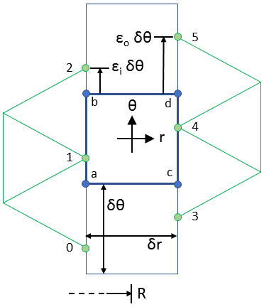
Figure 1: Problem definition for sliding band with linear interpolation.
These nodal values are interpolated from the edge values, \(A_0\), \(A_1\), and \(A_2\) on the inner edge and \(A_4\), \(A_5\), and \(A_6\) on the outer edge, using the linear interpolation in \(\ref{eqn1}\).
\[ \label{eqn1}
\begin{array}{ccc}
A_a & = & \epsilon_i A_0+ \left(1-\epsilon_i \right) A_1 \\
A_b & = & \epsilon_i A_1 + \left(1-\epsilon_i \right) A_2 \\
A_c & = & \epsilon_i A_3 + \left(1-\epsilon_i \right) A_4 \\
A_d & = & \epsilon_i A_4 + \left(1-\epsilon_i \right) A_5 \end{array} \]
The interpolation can be written more succinctly in matrix notation as:
\[ \label{eqn2} A_{abcd} = T_l \, A_{edge} \]
where \(A_{abcd}\) represents a vector of element unknowns and \(A_{edge}\) is a vector composed of \(A_0\) through \(A_6\) and linear interpolation matrix \(T_l\) is defined as:
\[ \label{eqn3} T_l = \left[
\begin{array}{cccccc}
\epsilon_i & 1-\epsilon_i & 0 & 0 &0 & 0 \\
0 & \epsilon_i & 1 - \epsilon_i & 0 & 0 & 0 \\
0 & 0 & 0 & \epsilon_o & 1-\epsilon_o & 0 \\
0 & 0 & 0 & 0 & \epsilon_o & 1-\epsilon_o \\
\end{array}
\right] \]
Matrix \(T_l\) is the mapping between edge and element nodes that can be used to represent the rectangular element matrix in terms of edge nodal values.
There are several valid approaches to deriving an element matrix for a rectangular element. Perhaps the simplest approach is the derivation of a rectangular element with piece-wise constant flux density (analogous to the piece-wise constant flux density of first-order triangular elements). An equation for the plane with the least-squares fit to the nodal values of A is:
\[ \label{eqn4}
A = \frac{1}{4} \left( A_a+A_b+A_c+A_d \right) + \frac{1}{2 \, \delta r} \left( A_c + A_d - A_a - A_b \right) (r-R) + \frac{1}{2\, \delta \theta} \left( A_b - A_a + A_d-A_c \right) \theta \]
where, without loss of generality, angle \(\theta\) is assumed to be zero at the center of the element. The relationship between vector potential, \(A\), and flux density, \(B\), in polar coordinates is [12]:
\[ \label{eqn7} {\bf B} = \frac{1}{r} \frac{\partial A}{\partial \theta} {\bf c}_r - \frac{\partial A}{\partial r} {\bf c}_\theta = B_r {\bf c}_r + B_{\theta} {\bf c}_\theta \]
Evaluating the flux density with \(A\) as defined by \(\ref{eqn4}\) yields \(\ref{eqn5}\) and \(\ref{eqn6}\), expressions for flux density in the element. Note that these expressions are constant over the element and not a function of position within the element.
\[ \label{eqn5} B_r = \frac{1}{2 \, R \delta \theta} \left( A_b - A_a + A_d-A_c \right) \]
\[ \label{eqn6} B_{\theta} = \frac{1}{2 \, \delta r} \left( A_a + A_b - A_c - A_d \right) \]
To derive the element matrix, the energy functional of the element is needed. Since there are no current sources in the gap, the energy functional (\(F\)) required to derive the finite element matrix via the calculus of variations is simply stored in the element:
\[ \label{eqn8} F = \frac{1}{2 \mu_o} \left( B_r^2 + B_{\theta}^2 \right) R \delta r \delta \theta \]
The element matrix (\(M_{lin}\)) is then obtained by taking partial derivatives of functional \(F\) with respect to each nodal value:
\[ \label{eqn9} M_{lin} = \frac{1}{4 \mu_o} \left[
\begin{array}{cccc}
k+k^{-1} & k^{-1}-k & k-k^{-1} & -k-k^{-1} \\
k^{-1}-k & k+k^{-1} & -k-k^{-1} & k-k^{-1} \\
k-k^{-1} & -k-k^{-1} & k+k^{-1} & k^{-1}-k \\
-k-k^{-1} & k-k^{-1} & k^{-1}-k & k+k^{-1}
\end{array} \right] \]
where \(k\) is the element's aspect ratio:
\[ \label{eqn10} k = \frac{\delta r}{R \delta \theta} \]
Element matrix \(M_{lin}\) is the element matrix in terms of the fixed element's nodal values. To obtain the element matrix in terms of rotor and stator edge nodal values, \(M_{lin}\) is pre- and post-multiplied by the transformation matrix (\(T\)) to obtain the linear interpolation sliding band element matrix, \(M_{sbl}\):
\[ \label{eqn11} M_{sbl} = T_l^T M_{lin} T_l \]
It can be noted every element in the band has the same element matrix; \(M_{sbl}\) need only be computed once, then applied to every element in the band.
The band of rectangular elements readily lends itself to torque computation via Arkkio's Method [14]. Arkkio's method essentially averages out all Maxwell Stress Tensor integration paths in a circular band in the air gap. Since each element has a piece-wise constant flux density, Arkkio's method reduces to a sum of flux density contributions from each element, as shown in \(\ref{eqn12}\). In \(\ref{eqn12}\), flux density is computed for each element from the mesh edge values using \(\ref{eqn5}\) and \(\ref{eqn6}\).
\[ \label{eqn12} \tau = R^2 \delta \theta \sum_{i=1}^n B_{\theta,i} B_{r,i} \]
Element matrix \(M_{sbl}\) in combination with torque computation via \(\ref{eqn12}\) results in a smooth computation of torque versus angular rotation. The scheme could therefore constitute an acceptable moving mesh approach. However, to compute BEMF, (numerical) differentiation of flux linkage with respect to rotor position is needed. From inspection of \(\ref{eqn11}\), it is clear that the element matrix varies continuously with rotor displacement for \(\epsilon_i\) and \(\epsilon_o\) on a range from 0 to 1. However, in the transition to the next set of elements (for motions larger than \(\delta \theta\)), there is no attribute that enforces continuity in the rate of change of the element matrix with respect to angular position across element transitions. The result is BEMF predictions that, while not grossly inaccurate, are not continuous across element transitions. To ensure continuity of computed BEMF, a higher order interpolation is needed.
Sliding Band with Cubic Interpolation
To pass through element transitions in a continuously differentiable fashion, element nodal values can be interpolated from mesh edge values using cubic Hermite splines. However, more boundary points are needed in order to create cubic Hermite splines. Figure 2 shows the cubic interpolation problem domain. Figure 2 shows that five points are used on either mesh boundary to interpolate the nodal values of the fixed rectangular elements in the band.
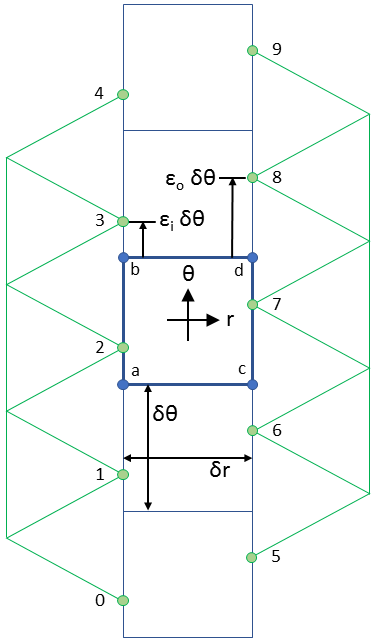
Figure 2: Problem definition for sliding band with cubic interpolation.
Cubic Hermite splines interpolate in a continuously differentiable way by interpolating based on both the function value and its derivative and the endpoints of each interval. [15] For example, as shown in Figure 3, node point \(A_a\) is interpolated from points \(A_0\), \(A_1\), \(A_2\), and \(A_3\).
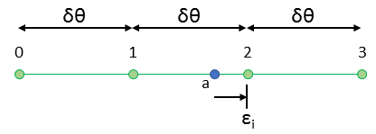
Figure 3: Interpolation of rectangular element node point \(a\).
For the cubic interpolation of the value at point \(a\), which lies between edge points \(1\) and \(2\), nodal values of \(dA/d\epsilon_i\) are needed. To ensure continuity with the next element, the derivative values are obtained from the neighboring nodal values using a centered difference scheme:
\[ \label{eqn13} \left( \frac{dA}{d\epsilon_i} \right)_1 = \frac{A_2 - A_0}{2} \]
\[ \label{eqn14} \left( \frac{dA}{d\epsilon_i} \right)_2 = \frac{A_3 - A_1}{2} \]
To derived the interpolation, edge nodes 1 and 2 are considered to be located at 0 and 1, respectively. Point \(a\) is located at \(1-\epsilon_i\). The solution for the cubic interpolation of \(A_a\) from the edge nodal values is given in \ref{eqn15}.
\[ \label{eqn15} A_a = \frac{1}{2} \left( (\epsilon_i-1) \epsilon_i^2 A_0 + \left(-3 \epsilon_i^3+4 \epsilon_i^2+ \epsilon_i \right) A_1 + \left((3 \epsilon_i - 5) e^2+2\right) A_2 - (\epsilon_i -1)^2 \epsilon_i A_3 \right) \]
The contribution of each edge node to \(A_a\) from \ref{eqn15} is shown below in Figure 4. At \(\epsilon_i=0\), node 2 directly maps to \(a\), and at \(\epsilon_i=1\), node 1 directly maps to \(a\). At the in-between points there is a small contribution from the "outboard" nodes that is needed to enforce continuity of the derivatives of each element' s contribution at the transitions between elements.
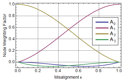
Figure 4: Contribution of each node to \(A_a\) vs. rotor position.
The contributions of each edge node can be rolled into a cubic interpolation version of the mapping matrix, \(T_c\), as shown in \(\ref{eqn16}\).
\[ \label{eqn16} T_c = \frac{1}{2} \left[
\begin{array}{cccc}
(\epsilon_i-1) \epsilon_i^2 & 0 & 0 & 0 \\
-3 \epsilon_i^3+4 \epsilon_i^2+\epsilon_i & (\epsilon_i-1) \epsilon_i^2 & 0 & 0 \\
3 \epsilon_i^3-5 \epsilon_i^2+2 & -3 \epsilon_i^3+4 \epsilon_i^2+\epsilon_i & 0 & 0 \\
-(\epsilon_i-1)^2 \epsilon_i & 3 \epsilon_i^3-5 \epsilon_i^2+2 & 0 & 0 \\
0 & -(\epsilon_i-1)^2 \epsilon_i & 0 & 0 \\
0 & 0 & (\epsilon_o-1) \epsilon_o^2 & 0 \\
0 & 0 & -3 \epsilon_o^3+4 \epsilon_o^2+\epsilon_o & (\epsilon_o-1) \epsilon_o^2 \\
0 & 0 & 3 \epsilon_o^3-5 \epsilon_o^2+2 & -3 \epsilon_o^3+4 \epsilon_o^2+\epsilon_o \\
0 & 0 & -(\epsilon_o-1)^2 \epsilon_o & 3 \epsilon_o^3-5 \epsilon_o^2+2 \\
0 & 0 & 0 & -(\epsilon_o-1)^2 \epsilon_o
\end{array}
\right]^T \]
The cubic sliding band element matrix, \(M_{sbc}\) is then obtained by pre- and post-multiplying by the cubic mapping matrix as in \(\ref{eqn17}\).
\[ \label{eqn17} M_{sbc} = T_c^T M_{lin} T_c\]
Matrix \(M_{sbc}\) is a \(10\times10\) symmetric matrix, but it is no more difficult to programmatically insert into the global stiffness matrix than any other sort of element matrix. Since the shift is the same for every element in the band, \(M_{sbc}\) need only be computed once, then applied to all elements in the band.
Alternate Rectangular Element Matrices
The \(M_{lin}\) matrix from \(\ref{eqn9}\) is perhaps the simplest element matrix for a rectangular element, but it is not the only possible rectangular element matrix. Two other choices for quadrilateral matrices that could replace \(M_{lin}\) in \(\ref{eqn11}\) and \(\ref{eqn17}\) are:
- Element matrix derived from a rectangle containing two first-order triangular elements. Under the "unrolled" geometry assumption, the quad element matrix derived from two triangles is as given in \(\ref{eqn18}\)
\frac{1}{2 \mu_o} \left[ \begin{array}{cccc}
k+k^{-1} & -k & -k^{-1} & 0 \\
-k & k+k^{-1} & 0 & -k^{-1} \\
-k^{-1} & 0 & k+k^{-1} & -k \\
0 & -k^{-1} & -k & k+k^{-1}
\end{array} \right] \]
Note that the use of this element matrix is not the same as the Moving Band methods. Although the elements in the band are effectively composed of triangles, the triangles do not deform as the rotor moves.
- Element matrix derived from a bilinear quadrilateral element. [16] Again, unrolling the band geometry, the element matrix is given by \(\ref{eqn19}\).
\begin{array}{cccc}
2 k+2 k^{-1} & k^{-1}-2 k & k-2 k^{-1} & -k-k^{-1} \\
k^{-1}-2 k & 2 k+2 k^{-1} & -k-k^{-1} & k-2 k^{-1} \\
k-2 k^{-1} & -k-k^{-1} & 2 k+2 k^{-1} & k^{-1}-2 k \\
-k-k^{-1} & k-2 k^{-1} & k^{-1}-2 k & 2 k+2 k^{-1}
\end{array} \right] \]
It is interesting to note that \(M_{bi}\) is a linear combination of \(M_{tri}\) and \(M_{lin}\):
\[ \label{eqn20} M_{bi} + \frac{1}{3} M_{tri} + \frac{2}{3}M_{lin} \]
The implication is that there is a family of possible quad element matrices that could be used, described by \(\ref{eqn21}\) and parameterized by variable \(c\). Parameter \(c\) is 0 for \(M_{lin}\), \(\frac{1}{3}\) for \(M_{bi}\) and 1 for \(M_{tri}\).
\[ \label{eqn21} M = c M_{tri} + (1-c) M_{lin} \]
Some other value of parameter \(c\) might be selected, for example to produce solutions that minimize the error with respect to a particular method of torque calculation.
Implementation in FEMM
FEMM [17] employs a Sliding Band formulation with cubic interpolation. For torque computation, FEMM employs a variation on \(\ref{eqn12}\). The program computes the flux density at the center of each element via \(\ref{eqn5}\) and \(\ref{eqn6}\), using the cubic mapping \(\ref{eqn16}\) to define nodal values in terms of edge values. However, FEMM does not compute the torque directly from nodal values as in \(\ref{eqn12}\). Instead, the program computes the Discrete Fourier Transform (DFT) of \(B_r\) and \(B_\theta\) and stores the coefficients of the transform. The coefficients allow continuous curves of \(B_r\) and \(B_\theta\) to be interpolated along the center line of the gap. The interpolated gap field is useful for both plotting and integration purposes.
Force and torque then computed by the program via Maxwell's Stress Tensor along the center line of the band elements by summing up contributions from each harmonic. For example, if \(b_r(i)\) and \(b_\theta(i)\) represent the complex-valued DFT coefficients for the \(i^{th}\) harmonic, the torque is:
\[ \label{eqn99} \tau = \frac{r}{4 \mu_o}\sum_{i=0}^n b_r(i) \bar{b_\theta}(i) + \bar{b_r}(i) b_\theta(i) \]
where \(n\) is the highest-numbered harmonic, computed from the number of points on the boundary and the periodicity of the domain. Eq. \(\ref{eqn99}]) gives a torque result that is very close (but not identical to) \(\ref{eqn12}]).
The a \(c\) coefficient for the element matrix in \(\ref{eqn21}\) was then selected to minimize the error in \label{eqn99} on a problem with an analytical solution for torque. [18] The error-minimizing value of \(c\) determined from the benchmark problem is \(c=\frac{2}{3}\).
Numerical Examples
As a numerical example, the brushless DC (BLDC) motor geometry from [8] is used to compare:
- A Moving Band scheme implement with 1st order triangles (for reference);
- A Sliding Band scheme with linear interpolation as described by \(\ref{eqn17}\)
- The FEMM baseline cubic Sliding Band implementation described in the previous section.

Figure 5: BLDC example from [8].
Relevant geometry was gleaned from Fig. 4 in [8]. The materials and axial length were selected to yield a line-to-line voltage whose amplitude is a match to that in Fig. 5 of [1]. A detailed list of the derived dimensions and materials is shown below in Table 1.
| Attribute | Value |
| Rotor Inner Diameter | 22.8mm |
| Rotor Iron Outer Diameter | 50.5mm |
| Rotor Outer Diameter | 55.1mm |
| Magnet Width | 15.8566mm |
| Air Gap Length | 0.7mm |
| Angle Spanned by Tooth | 11.9deg |
| Tooth width | 4mm |
| Tooth Root diameter | 86.592mm |
| Stator Outer Diameter | 100mm |
| Turns/Slot | 46 |
| Winding Wire | 4X20AWG copper wire |
| Magnet Material | Sm2Co17 24MGOe |
| Stator Material | 24 Gauge M19 NGO Steel @ 98% fill |
| Rotor Material | 1018 steel |
| Axial Length | 50mm |
To compare various movement methods, the no-load line-to-line voltage was obtained using \(5 \mu s\) time steps for a machine running at 2000rpm, implying a 0.06 degree step in position (i.e. the same simulation considered in [8]). A 1977 node mesh was employed with elements in the gap spanning 0.6 degrees. This element size provides 10 position steps per mesh element). A close-up of the mesh is shown in Figure 6 below.

Figure 6: Mesh has 0.6 degree spacing along the air gap.
As in [8], some 2000 simulations were performed over 120 degrees of rotor motion. A list of flux linkage versus time for each phase was interpolated using Mathematica's Interpolation function with linear interpolation between points. The interpolating functions were then analytically differentiated with respect to time to yield line-to-neutral voltage. The difference between line-to-neutral voltages was taken to yield line-to-line voltage.
The complete simulated line-to-line voltage from FEMM is shown in Figure 7. However, the graph must be zoomed to a small section to see the difference between the performance of various motion strategies.
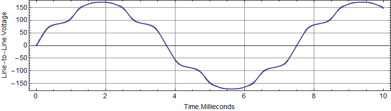
Figure 7: Simulated and benchmark line-to-line voltage for a BLDC machine from [1].
Figure 8 shows a close-up of the flat section of Figure 7 in the region around 3ms.

Figure 8: Detail of simulated line-to-line voltage for various movement schemes].
The small-scale steps in all plots represent the numerical differentiation of data taken at 0.06 degree increments. The larger jump in the 1st order Sliding Band (blue line) represents the transition to the next group of elements. The larger jumps in the 1st order Moving Band (magenta line) represent the points at which a remeshing occurred; at intermediate points, the mesh is deformed rather than remeshed. In contrast, the cubic Sliding Band (the baseline implementation in FEMM) is smooth with no element transitions in evidence.
Conclusions
A novel approach to modeling rotor motion in a finite element mesh has been presented. The level of implementation effort is equivalent to the widely-used 1st order Moving Band method. However, the new method provides a continuous estimate of back EMF, whereas the BEMF predicted by Moving Band has small jumps coinciding with remeshing. The new method is implemented in the FEMM as of the 25Feb2018 test build.
References
[1] C. Bernardi, Y. Maday, and F. Rapetti, "Basics and some applications of the mortar element method," GAMM-Mitteilungen 28(2):97-120, Nov. 2005 .
[2] O. J. Antunes et al., "Using hierarchic interpolation with mortar element method for electrical machines analysis," IEEE Transactions on Magnetics, 41(5):1472-1475, May 2005.
[3] D. Rodger, H. C. Lai, and P. J. Leonard, "Coupled elements for problems involving movement," IEEE Transactions on Magnetics, 26(2):548-550, Mar. 1990.
[4] O. J. Antunes et al., "Comparison between nonconforming movement methods," IEEE Transactions on Magnetics, 42(4):599-603, Apr. 2006.
[5] R. Perrin-Bit and J. L. Coulomb, "A three dimensional finite element mesh connection for problems involving movement," IEEE Transactions on Magnetics, 31(3):1920-1923, May 1995.
[6] D. Marcsa, "Rotational motion modelling for numerical analysis of electrical machines," Acta Technica Jaurinensis, 10(2):437-450, June 2017.
[7] M. V. Ferreira da Luz et al. "Analysis of a permanent magnet generator with dual formulations using periodicity conditions and moving band," IEEE Transactions on Magnetics, 38(2):961-964, Mar. 2002.
[8] O. J. Antunes, J. P. A. Bastons, and N. Sadowski, "Using high-order finite elements in problems with movement," IEEE Transactions on Magnetics, 40(2):529-533, Mar. 2004
[9] S. Gerber and R-J. Wang, "Implementation of a moving band solver for finite element analysis of electrical machines," Proc. 22nd South African Power Engineering Conference, pp249-254, Durban, 30-31 January 2014
[10] A. A. Abdel-Razek et al., "Conception of an air-gap element for the dynamic analysis of the electromagnetic field in electric machines," IEEE Transactions on Magnetics, 18(2):655-659, Mar. 1982.
[11] H. De Gersem and T. Weiland, "A computationally efficient air-gap element for 2-D FE machine models," IEEE Transactions on Magnetics, 41(5):1844-1847, May 2005.
[12] H. A. Haus and J. R. Melcher, Electromagnetic Fields and Energy, Prentice-Hall, 1989.
[13] S. R. H. Hoole, Computer-aided analysis and design of electromagnetic devices, Elsevier, 1989.
[14] A. Arkkio, Analysis of induction motors based on the numerical solution of the magnetic field and circuit equations, (Doctoral dissertation) Helsinki University of Technology, 1987
[15] Wikipedia "Cubic hermite splines," Wikipedia, https://en.wikipedia.org/wiki/Cubic_Hermite_spline, accessed 10Mar2018.
[16] P. I. Kattan, MATLAB Guide to Finite Elements, Springer, 2008.
[17] D. Meeker, Finite Element Method Magnetics (FEMM), 25Feb2018 build
[18] D. Meeker, "(Anti)Periodic Air Gap Boundary Condition Torque Benchmark", 25Feb2018.
| File | Last modified | Size |
|---|---|---|
| SlidingBand.pdf | 2018-04-09 21:56 | 410Kb |